| Issue |
A&A
Volume 673, May 2023
|
|
|---|---|---|
| Article Number | A100 | |
| Number of page(s) | 16 | |
| Section | Extragalactic astronomy | |
| DOI | https://doi.org/10.1051/0004-6361/202346119 | |
| Published online | 12 May 2023 | |
A UNIONS view of the brightest central galaxies of candidate fossil groups⋆,⋆⋆
1
Sorbonne Université, CNRS, UMR 7095, Institut d’Astrophysique de Paris, 98bis Bd Arago, 75014 Paris, France
e-mail: chu@iap.fr
2
Anton Pannekoek Institute for Astronomy & GRAPPA, University of Amsterdam, Science Park 904, 1098 XH Amsterdam, The Netherlands
3
IRAP, Institut de Recherche en Astrophysique et Planétologie, Université de Toulouse, UPS-OMP, CNRS, CNES, 14 avenue E. Belin, 31400 Toulouse, France
4
Aix-Marseille Univ., CNRS, CNES, LAM, 13388 Marseille, France
5
Instituto de Astrofísica de Andalucía, CSIC, Glorieta de la Astronomía s/n, 18008 Granada, Spain
6
Institute for Astronomy, University of Hawaii, 2680 Woodlawn Drive, Honolulu, HI 96822, USA
7
Université Paris-Saclay, Université Paris Cité, CEA, CNRS, AIM, 91191 Gif-sur-Yvette, France
8
Herzberg Astronomy and Astrophysics, National Research Council, 5071 West Saanich Road, Victoria, BC V9E2E7, Canada
Received:
10
February
2023
Accepted:
7
March
2023
Context. The formation process of fossil groups (FGs) is still under debate, and, because of their relative rarity, large samples of such objects are still missing.
Aims. The aim of the present paper is to increase the sample of known FGs, to analyse the properties of their brightest group galaxies (BGGs), and to compare them with a control sample of non-FG BGGs.
Methods. We extracted a sample of 87 FG and 100 non-FG candidates from a large spectroscopic catalogue of haloes and galaxies. For all the objects with data available in UNIONS (initially the Canada France Imaging Survey, CFIS) in the u and r bands, and/or in an extra r-band processed to preserve all low-surface-brightness features (rLSB), we performed a 2D photometric fit of the BGG with GALFIT with one or two Sérsic components. We also analysed how the subtraction of the intracluster light (ICL) contribution modifies the BGG properties. From the SDSS spectra available for the BGGs of 65 FGs and 82 non-FGs, we extracted the properties of their stellar populations with Firefly. To complement our study, and in order to provide a detailed illustration of the possible origin of emission lines in the FG BGGs, involving the presence or absence of an AGN, we investigated the origin of the emission lines in a nearby FG that is dominated by the NGC 4104 galaxy.
Results. Morphologically, a single Sérsic profile can fit most objects in the u band, while two Sérsics are needed in the r and rLSB bands, both for FGs and non-FGs. Non-FG BGGs cover a larger range of Sérsic index n. FG BGGs follow the Kormendy relation (mean surface brightness versus effective radius) previously derived for almost 1000 brightest cluster galaxies (BCGs), while the majority of non-FGs BGGs are located below this relation, with fainter mean surface brightnesses. This suggests that FG BGGs have evolved similarly to BCGs, and non-FG BGGs have evolved differently from both FG BGGs and BCGs. All the above properties can be strongly modified by the subtraction of the ICL contribution. Based on spectral fitting, the stellar populations of FG and non-FG BGGs do not differ significantly.
Conclusions. FG and non-FG BGGs differ from one another in terms of their morphological properties and Kormendy relation, suggesting they have had different formation histories. However, it is not possible to trace differences in their stellar populations or in their large-scale distributions.
Key words: galaxies: clusters: general / galaxies: evolution / galaxies: formation / galaxies: groups: general
Data of the two samples of 87 fossil groups and 100 non fossil groups are only available at the CDS via anonymous ftp to cdsarc.cds.unistra.fr (130.79.128.5) or via https://cdsarc.cds.unistra.fr/viz-bin/cat/J/A+A/673/A100
© The Authors 2023
 Open Access article, published by EDP Sciences, under the terms of the Creative Commons Attribution License (https://creativecommons.org/licenses/by/4.0), which permits unrestricted use, distribution, and reproduction in any medium, provided the original work is properly cited.
This article is published in open access under the Subscribe to Open model. Subscribe to A&A to support open access publication.
1. Introduction
Fossil groups (FGs) were discovered by Ponman et al. (1994). They are particular groups of galaxies with high X-ray luminosities but with fewer bright galaxies than most groups or clusters of galaxies. Jones et al. (2003) later provided a commonly accepted definition of FGs based on the satisfaction of three conditions: they are extended X-ray sources with an X-ray luminosity of at least LX = 1042 h erg s−1; with a brightest group galaxy (BGG) at least two magnitudes brighter than other group members; and the distance between the two brightest galaxies must be smaller than half the group virial radius. The formation mechanism of these peculiar objects and why they present such a low amount of optically emitting matter are still under debate. Jones et al. (2003) suggested that FGs are the remnants of early mergers, and that they are cool-core structures that accreted most of the large galaxies in their environment a long time ago, a scenario supported by hydrodynamical simulations by D’Onghia et al. (2005). However, FGs could also be a short temporary stage of group evolution before they capture more galaxies in their vicinity, as reported for instance by von Benda-Beckmann et al. (2008) based on N-body simulations.
FGs can be studied through their optical (Vikhlinin et al. 1999; Santos et al. 2007) or X-ray properties (Romer et al. 2000; Adami et al. 2018). Some optical studies support the scenario that FGs are the result of a large amount of dynamical activity at high redshift, but in an environment that is too poor for them to evolve into a cluster of galaxies through the hierarchical growth of structures. For example, La Barbera et al. (2009) found that the optical properties of BGGs in FGs are identical to those of giant isolated field galaxies. Girardi et al. (2014) found a similar relation between their X-ray and optical luminosities for FGs and for normal groups, suggesting that all groups contain the same amount of optical material, but that in FGs it is concentrated in a giant central elliptical galaxy that has cannibalised most of the surrounding bright galaxies. At X-ray wavelengths, based on Chandra X-ray observations, Bharadwaj et al. (2016) found that FGs are mostly cool-core systems, suggesting that these structures are no longer dynamically active.
However, recent observations tend to contradict the findings that FGs are dynamically relaxed systems that have not undergone recent merging events. For example, Kim et al. (2018) reported that the prototypical FG NGC 1132 shows an asymmetrical disturbed X-ray profile, and suggested that it is dynamically active. Similarly, Lima Neto et al. (2020) detected shells around the BGG of NGC 4104 and, based on N-body simulations, showed that this FG probably experienced a relatively recent merger between its BGG and another bright galaxy with a mass of about 40% of that of the BGG. More details on FGs can be found in the recent review by Aguerri & Zarattini (2021).
To make up for the lack of large samples of FGs, Adami et al. (2020) carried out a statistical study of FGs, extracted from the catalogue of 1371 groups and clusters detected by Sarron et al. (2018) in the Canada-France-Hawaii Telescope Legacy Survey (CFHTLS). These systems were detected based on photometric redshifts (Ilbert et al. 2006). Adami et al. (2020) found that groups with masses larger than 2.4 × 10¹⁴ M⊙ have the highest probability of being FGs and discussed their location in the cosmic web relative to nodes and filaments (for a similar study, see also Zarattini et al. 2022). Adami et al. (2020) concluded that FGs were most probably in a poor environment, making the number of nearby galaxies insufficient to compensate for the accretion by the central group galaxy.
Numerical simulations of FGs by Dariush et al. (2007) showed good agreement with both optical and X-ray observations, and predicted that fossil systems will be found in significant numbers (3%–4% of the population), even for relatively rich clusters. These authors find that FGs assemble a higher fraction of their mass at high redshifts than non-FGs, with the ratio of the currently assembled halo mass to final mass, at any epoch, being about 10%–20% higher for FGs. Their interpretation is that FGs represent undisturbed, early-forming systems in which large galaxies have merged to form a single dominant elliptical.
The role of the BGG is therefore crucial in explaining the lack of bright galaxies in FGs. The aim of the present paper is to analyse the physical properties of the BGGs of FGs and compare them to those of non-FGs and clusters. For this, we gathered as large a sample of FGs as possible from the sample of groups detected by Tinker1 from SDSS data (Sect. 2). In each FG candidate, we detected the BGG and measured its morphological properties. We then compared the properties of FG BGGs to those of a control sample of non-FGs, as well as to the brightest galaxies of clusters and massive groups of galaxies previously studied by Chu et al. (2021, 2022) to study how FG BGGs compare to the BCGs and BGGs of more imposing systems (Sect. 3). We also analysed the stellar populations of FG and non-FG BGGs and investigated the origin of the BGG spectroscopic emission lines, taking as an example the BGG of a very nearby FG, NGC 4104 (Sect. 4). Finally, our results are discussed in Sect. 5.
2. Data
2.1. Selection of FGs
Tinker has made catalogues available that contain data for 559 038 galaxies. Among other quantities, these catalogues provide positions, spectroscopic redshifts from the SDSS survey, k-corrected and evolution-corrected (to z = 0.1) g and r band absolute magnitudes, galaxy stellar masses, and total halo masses. For each galaxy, the group to which it belongs is indicated.
The group-finding algorithm described by Tinker (2021) is based on the halo-based group finder of Yang et al. (2005), which was further vetted by Campbell et al. (2015). The standard implementation of the group finder yields central galaxy samples with a purity and completeness of 85%–90% (Tinker et al. 2011). To assign stellar masses to haloes and subhaloes, Tinker (2021) uses the stellar mass function from Cao et al. (2020), which takes into account the principal component analysis galaxy stellar masses of Chen et al. (2012).
We first eliminated all the galaxies that were alone in a group – because a single galaxy in a halo does not form a group – and obtained a catalogue of 201 007 galaxies that were at least in a pair. We then selected the galaxies belonging to groups where the magnitude difference in the r band between the brightest and second-brightest galaxy was at least 2 mag, and for which the distance between these two galaxies was smaller than half the virial radius, Rvirial:

where the corresponding mass Mhalo is given in the Tinker catalogue, and H(t) the Hubble constant at the group redshift. We thus obtained a catalogue of 2453 galaxies. We note that in this process, we do not take into account the possibility to have a projected galaxy at less than half the virial radius, which could physically (in 3D) be at more than half the virial radius (because of the lack of precision of the spectroscopic redshift or because of high proper velocity). Such a galaxy could artificially be placed in the group luminosity function between the BGG and the second ranked galaxy, and therefore disqualify the group as a FG. However, such a case would simply limit the size of our sample, which would eliminate some of the genuine FGs. This effect will not pollute our FG sample by inserting non-FGs.
From the above catalogue, we extracted a list with the brightest galaxy of each group, and this led to a catalogue of 1112 galaxies that may be considered as BGGs. This means that most groups were made of pairs. In order to avoid considering objects that could not be real groups, such as isolated galaxies with a few small satellites, we added a condition on the halo mass: Mhalo > 1013 M⊙, giving 88 FG candidates. This limit was chosen to match the lowest mass that we found for a FG in our search for FGs in the CFHTLS: 1.1 × 10¹³ M⊙ (Adami et al. 2020). In the absence of X-ray data for all but one of our objects, this condition also gives us more confidence that these systems may indeed be FGs. Indeed, N. Clerc kindly matched our FG catalogue with his XCLASS catalogue of X-ray sources derived from XMM-Newton data and only found one match for FG17 (e.g. FG #17 of Table A.1), with LX = 5 × 1041 h erg s−1 in the [0.5–2] keV energy band. This value is slightly lower than the limit of 1042 h
 erg s−1 defined by Jones et al. (2003). For the other FGs, this does not mean that they are not X-ray emitters, but simply that they are not located in regions observed by XMM-Newton.
The last step was to use photometric catalogues from UNIONS2 to verify that no galaxies were missed in spectroscopy. The Ultraviolet Near Infrared Optical Northern Survey (UNIONS) collaboration combines wide-field imaging surveys of the northern hemisphere. UNIONS consists of the Canada-France Imaging Survey (CFIS), conducted at the 3.6 meter CFHT on Maunakea, parts of Pan-STARRS, and the Wide Imaging with Subaru HyperSuprime-Cam of the Euclid Sky (WISHES). CFHT/CFIS is obtaining deep u and r bands; Pan-STARRS is obtaining deep i and moderate-deep z band imaging, and Subaru is obtaining deep z-band imaging through WISHES and g-band imaging through the Waterloo-Hawaii IfA g-band Survey (WHIGS). These independent efforts are designed, in part, to secure optical imaging in order to complement the Euclid space mission, although UNIONS is a separate collaboration designed to maximise the science return of these large and deep surveys of the northern skies.
We searched the UNIONS photometric archive for objects (galaxies or stars) that (1) fall within 0.5 × Rvirial of a FG centre, (2) are missing from the Tinker catalogue, and (3) have magnitudes between that of the BGG and that of the second brightest galaxy. Stars were removed with central surface brightness versus total magnitude plots.
2.2. Additional spectroscopic observations of fossil group
At the end of this selection process, we found three galaxies not present in the Tinker spectroscopy and potentially falling within two magnitudes from the BGG. This affected two FG candidates: FG65 and FG73 (see Table A.1).
For FG65, we obtained long-slit spectroscopy with MISTRAL at Observatoire de Haute-Provence for the two relatively bright galaxies (RA = 228.7630093°, Dec = 42.0503814° and RA = 228.769596°, Dec = 42.0548771°, 1 hour exposures), which both have magnitudes differing by less than 2 mag from the BGG. Both proved to be part of the same foreground galaxy at z = 0.0149, and not related to the FG BGG at z = 0.13479. This confirmed the fossil nature of the FG65 group.
We also observed a galaxy (RA = 238.45581°, Dec = 56.4229°, 1 h exposure) within the FG73 FG candidate with CAFOS at the Calar Alto Hispano Alemán Telescope. This galaxy was found to be at a redshift of 0.1055, which is very close to the redshift of the putative BGG (z = 0.1080), and to be different from the BGG by less than 2 mag. FG73 was therefore removed from the FG final list because the two-magnitudes difference criterium between the brightest and second-brightest galaxies is not satisfied. We thus obtained the final catalogue of 87 FG candidates listed in Table A.1.
2.3. Basic properties of fossil groups
The histograms of the halo masses and BGG stellar masses of the FG candidates and of the comparison sample (see below) are shown in Figs. 1 and 2, respectively. These quantities are taken from the Tinker catalogues. The halo masses are in the [1013,1014] M⊙ range, with 65 FGs (74%) having halo masses ≤2 × 10¹³ M⊙. The BGG stellar masses are in the [1010.8,1012] M⊙ range, except for one galaxy (FG22), which has a lower mass of 1010.4 M⊙.
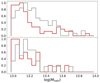 |
Fig. 1. Normalised histograms of the logarithms of the halo masses for FGs (red) and non-FGs (grey). Top: 87 FGs and 100 non-FGs. Bottom: 25 FGs and 30 non-FGs analysed morphologically. |
The redshift histogram of the groups is shown in Fig. 3. Most of the FGs are in the [0.02,0.12] range, with only five FGs in the [0.12,0.18] range. The absolute magnitude histograms in the g and r bands, together with the (g–r) colour histogram, are shown in Fig. 4 for the groups. BGGs have typical absolute magnitudes in the r band in the [−23, −21] range, with typical (g–r) colours in the [0.8,1.0] range.
We searched for images of these 87 FG candidates in the UNIONS image database in the u and r bands. These images were retrieved from the DR3, which includes observations made before January of 2021, and covers 7000 deg2 in u and 3600 deg2 in r. We found images for 35 FGs in the u band and for 25 FGs in the r band, among which 12 FGs having both u and r band images. We indicate in Table A.1 (last column) the FGs with UNIONS images available.
Chu et al. (2022) show that subtracting the contribution of intracluster light (ICL) could modify the properties derived for BCGs. Therefore, with the aim of estimating how subtracting the ICL could modify the properties derived for the BGG, we also exploited the r band images processed to preserve all low-surface-brightness (LSB) features (hereafter referred to as rLSB). As explained by Žemaitis et al. (2023), for example, the images were obtained using an observing technique that is optimised for LSB surveys at CFHT (e.g. Ferrarese et al. 2012; Duc et al. 2015).
There were 19 FGs available in rLSB. For all these objects, we extracted images of 4000 × 4000 pixels2 centred on the BGG, either by cropping the tiled UNIONS rLSB images, or by first assembling two to four tiled images with the SExtractor and SWarp softwares (Bertin & Arnouts 1996; Bertin et al. 2002; Bertin 2006)3 and then cropping them to this size. In the latter case, special care was taken to assemble tiles that had been background subtracted in order to avoid losing faint signal in the outskirts of BGGs.
2.4. Control sample of non-fossil groups
In order to compare the properties of BGGs of FGs with those of non-FGs, we built a catalogue of non-FGs in a similar way, but this time imposing a magnitude difference between the brightest and second-brightest galaxies of smaller than 2. This condition, together with that of Mhalo > 1013 M⊙, gave 100 non-FG candidates; none of these has a match in the XCLASS X-ray catalogue of N. Clerc.
The catalogues of the 87 FG candidates and of the 100 non-FGs are available in electronic form at the CDS, and contain the following columns: number, RA, Dec, spectroscopic redshift, BGG stellar mass, absolute magnitude in the g and r SDSS bands, virial radius, and halo mass. Among the 100 non-FGs, we chose 30 non-FGs with good-quality UNIONS images in u, r, and rLSB. These objects are listed in Table A.2. This subsample of non-FGs is comparable in number to that of the FG candidates for which UNIONS data are available. The BGGs of this control sample were chosen to match the absolute magnitude and colour histograms of our FG sample as closely as possible. This can be checked by looking at Figs. 1–4. A Kolmogorov-Smirnov test on the FG and non-FG samples shows that these two samples have only a 40% probability of being statistically different.
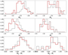 |
Fig. 4. Normalised histograms of the absolute magnitudes of the BGGs in the g (top) and r (middle) bands, and of the (g − r) colour (bottom) for FGs (red) and non-FGs (grey). Left: 87 FGs and 100 non-FGs. Right: 25 FGs and 30 non-FGs analysed morphologically. |
For each FG and non-FG, we extracted all the galaxies belonging to the same halo within 1 arcmin around the BGG from the Tinker catalogue (which gives absolute magnitudes in the g and r bands). The colour–magnitude diagram shown in Fig. 5 shows that all FG BGGs follow a very well-defined sequence. With a colour of g − r = −1.29, only one BGG is bluer than g − r = 0 and falls outside the plot; it appears to be a spiral galaxy, but we kept it in the sample. BGGs of non-FGs surprisingly follow this sequence very well, whereas the galaxies that are not BGGs tend to be fainter and show a notably larger dispersion.
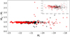 |
Fig. 5. (g − r) colour magnitude diagram for four samples: light red dots: galaxies within 1 arcmin of FG BGGs; red stars: FG BGGs; grey dots: all galaxies within 1 arcmin of non-FG BGGs; black stars: non-FG BGGs. The x-axis is the absolute magnitude in the r band. A zoomed-in version of the plot at the brightest magnitudes is shown in the top right corner. |
3. Morphological properties of the FG BGGs
3.1. Method
We now consider the 25 and 30 BGGs of FGs and non-FGs for which r band data are available in UNIONS. Following Chu et al. (2021) and Chu et al. (2022), the 2D profile of each BGG was fit with GALFIT (Peng et al. 2002) with a single Sérsic model and with a double Sérsic model. GALFIT initial parameters were obtained with SExtractor using a bulge + disk model. A mask and a point spread function were created following the method described in Chu et al. (2021). The choice between a single and double Sérsic model was made based on the statistical F-test (Margalef-Bentabol et al. 2016) and the computed p-value, which indicates whether or not complexifying the model is necessary by increasing the number of degrees of freedom. As the current sample has the same resolution as that of Chu et al. (2022), we adopt the same p-value limit to distinguish between the two different models: P0 = 0.15.
3.2. Morphological properties of fossil groups
The numbers of BGGs of FGs and non-FGs for which one Sérsic law (S1) or two Sérsic laws (S2) are needed to fit their 2D profiles in the various bands are given in Table 1. For FGs, we can see that in the u band, most BGGs can be fit with a single Sérsic (83%). In contrast, a major part of the profiles in the r band require two components (92%). If we now consider the BGGs from the rLSB data, only 53% require two Sérsics.
2D profile model distribution of BGGs of FGs and non-FGs.
The fact that a single Sérsic fits most of the u band images of BGGs could be due to the lower signal-to-noise ratio (S/N) in the u band, which makes the detection of a faint outer component difficult, while this outer LSB component is better detected in the deeper r band images. In line with this interpretation, it appears surprising that the percentage of BGGs better fit by two Sérsics is smaller in the deeper rLSB data than in the r band data. This can be explained by the fact that the Elixir-LSB pipeline, during the refined background-subtraction procedure, removes light from around the BGGs. We cannot guarantee whether this light originates from the BGG, is due to instrumental contamination, or a mixture of both. This nevertheless means that part of our two Sérsic fits in the r band is potentially contaminated by MegaCam scattered light. We decided to keep both bands for comparison purposes: the r band, with more flux but potentially contaminated, and the rLSB band that is ‘cleaner’ but might be missing light from the BGG outer profiles.
The same 2D profile fitting was applied to the control sample of non-FGs. As for FGs, we see in Table 1 that most BGGs in the u band are fit with a single Sérsic (90%) while in the r band 80% are better fit with two Sérsics, and in rLSB, 53% are better fit with two Sérsics. The difference between FGs and non-FGs is therefore of a few percent, a value that is not significant in view of the dispersion.
As described in Sect. 3.4, we computed the ICL contribution and subtracted it from the BGGs to see how the Sérsic parameters changed. If we look at Table 1, we can see that only 3 FG BGGs out of 19 (16%) can be fit with a single Sérsic, and for non-FG BGGs, 6 out of 30 BGGs (20%) are fit with a single Sérsic. The subtraction of the ICL contribution therefore does not make the second Sérsic component disappear, as already observed by Chu et al. (2022). The effect of ICL on the morphological properties of BGGs is further discussed in Sect. 3.4. Unexpectedly, we find more BGGs of FGs and non-FGs that are better modelled by two-Sérsic profiles on ICL-subtracted rLSB images than on rLSB images. This is discussed in Sect. 5.
As seen in Fig. 6, the effective radii are comparable for the BGGs of FGs and non-FGs in all filters. The absolute magnitudes of FG BGGs appear brighter (by up to one magnitude) than those of non-FG BGGs. The same is observed for the mean surface brightnesses, except in the u filter, where they appear similar.
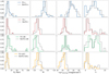 |
Fig. 6. Normalised histograms of the effective radius, absolute magnitude, mean surface brightness corrected for cosmological dimming, and Sérsic index n (from left to right). From top to bottom: 35 candidate FGs (in blue) and 30 non-FGs (grey) in the u band; 25 candidate FGs (in red) and 30 non-FGs (grey) in the r band; 19 candidate FGs (green) and 30 non-FGs (grey) in the rLSB band; same as above in the rLSB band after ICL subtraction (yellow for FGs). |
The histograms of the Sérsic indices n are more concentrated towards low values in r for FGs: only 2 FGs out of 25 (8%) have n > 4, while 8 non-FGs out of 30 (27%) have n > 4. In rLSB, there are 10 FGs out of 19 (53%) and 18 non-FGs out of 30 (60%) with n > 4. This high value of n may be linked to the presence of ICL (see Sect. 3.4).
Because the difference in Sérsic indices between FGs and non-FGs is not apparent in all bands, and the effective radii are approximately the same, the only clear difference that we find between the physical properties of FGs and non-FGs is that FG BGGs are intrinsically brighter. This may be due to a selection bias, as our sample of FG BGGs is overall brighter than our sample of non-FG BGGs (see Fig. 4). Despite our efforts to build two samples with similar properties, we could not find as many non-FG BGGs that are as bright as FG BGGs. This may indicate that, in a given group-mass range, FG BGGs are indeed brighter and most of the mass of the group is concentrated in the BGG.
3.3. Kormendy relation
We now consider the relation found by Kormendy (1977) (mean effective brightness ⟨μ⟩ as a function of effective radius Re), which can be fit with the following law:

The slopes and intercepts with their errors are given in Table 2 in the u, r, rLSB and ICL-subtracted rLSB bands, both before and after correction for cosmological dimming applied as in Chu et al. (2022). For better comparison with this latter study, we converted the surface brightnesses measured in the u, r, rLSB and ICL-subtracted rLSB bands into those in the i band using the Fukugita et al. (1995) tables. We can see in Table 2 that the dispersion is smaller for FGs than for non-FGs in all bands, and that the relations in u and r are parallel within the dispersion. With the exception of the rLSB band, the slopes are larger for non-FGs than for FGs, but in view of the dispersion this difference is not significant.
Kormendy relation of BGGs of FGs and non-FGs.
The Kormendy relation derived in the i band for almost 1000 BCGs by Chu et al. (2022) was ⟨μ⟩=(3.34 ± 0.05)×log(Re)+(18.65 ± 0.07) and ⟨μ⟩=(3.49 ± 0.04)×log(Re)+(16.72 ± 0.05) before and after correction for cosmological dimming, respectively. This relation was found to be independent of the model used (one or two Sérsic profiles). If we compare the Kormendy relations found here for FGs and non-FGs to those of Chu et al. (2022), we see that FGs are located on this relation, while the majority of non-FGs are located below the relation, as illustrated in Fig. 7, and this is true both before and after ICL subtraction. However, in view of the large dispersion, the difference in the intercepts is not statistically significant.
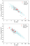 |
Fig. 7. Kormendy relation for FGs in red and non-FGs in grey, superimposed on the relation found for almost 1000 BCGs by Chu et al. (2022) in cyan. Both plots are obtained in the rLSB band, the top plot without ICL subtraction and the bottom plot after ICL subtraction. The points for FGs and non-FGs have been shifted from the r to the i band, and all points are corrected for cosmological dimming. |
Therefore, the BGGs of FGs appear to have properties more similar to those of BCGs than to those of non-FG BGGs, suggesting that BGGs in FGs and BCGs have followed a comparable evolutionary path, while non-FGs have evolved somewhat differently, reaching fainter surface brightnesses.
3.4. Influence of the ICL contribution on the estimation of the morphological properties of FGs
Chu et al. (2022) estimated the importance of the ICL contribution for the morphological properties of seven BCGs computed with GALFIT. To this end, these authors fitted the 2D properties of the BCGs to the original images, and then subtracted the contribution of the ICL derived by Jiménez-Teja et al. (2018) from these images before fitting the BCGs again. The main result of Chu et al. (2022) was that two Sérsics were still necessary to fit the BCGs, and therefore that the need for a second component could not only be attributable to ICL. In all cases, the effective radii increase in the presence of ICL, some of them drastically (by an order of magnitude). For all seven BCGs, the absolute magnitude of the external component is fainter after removing the ICL (with a difference that can reach two magnitudes). After subtracting ICL, BCGs also have brighter effective surface brightnesses, with a difference that can almost reach 3 mag arcsec−2.
Similarly, to better quantify the effect of the ICL in the present study, we now compare the values of the various physical parameters galaxy by galaxy before and after ICL subtraction. This demands an estimation of the ICL contribution for each FG. For this, we use DAWIS (Detection Algorithm with Wavelets for Intracluster light Studies; Ellien et al. 2021), a wavelet-based algorithm optimised for the detection and characterisation of LSB structures in deep optical images. Briefly, DAWIS applies a wavelet transform to the analysed image and detects sources in the new wavelet representation. The light profiles in the original image of these sources are then modelled from their wavelet representation through a restoration procedure. DAWIS follows a semi-greedy procedure, meaning that sources are restored iteratively. The brightest detected sources are modelled first and removed from the image, and the whole wavelet procedure is then applied again on the residual image. New sources are detected, modelled and removed, until convergence to a noise only residual map. This provides a refined modelling of all detected sources, from very bright objects down to very faint structures. We note that the detected sources are not necessarily entire astrophysical objects, but rather substructures of such objects. DAWIS was applied to each FG for which we have an image in the rLSB band, providing for each of them a list of sources and their light profiles.
For each BGG, from the DAWIS output list, we extracted a sublist of sources that are identified as contributing to ICL. This sublist was estimated using the following criteria: the source must be unimodal and centred on the BGG centre, and its spatial radial extent must be greater than or equal to a given radius. We tried different values for the spatial extent, going from 40 kpc up to 100 kpc. Low values lead to brighter ICL contribution, contaminated by smaller sources such as pieces of foreground and background galaxies. For our study, we chose to remove a clean ICL contribution, potentially missing some of it, rather than a contribution contaminated by galaxies, and set the radius to 100 kpc. The light profiles of these sources are summed into a 2D ICL profile, and this profile is then subtracted from the BGG light profile. More details about this procedure and DAWIS can be found in Ellien et al. (2021) and Brough et al. (in prep.).
The results after ICL subtraction are illustrated in Fig. 8 and Table 3. We can see that for FGs, the ICL increases the effective radius by a mean factor of 3.7, and the ICL adds light to the BGG by up to 1.3 mag. With ICL, the mean surface brightness can be up to 5 mag arcsec−2 brighter, with a mean at 1.3, and the Sérsic index n tends to be larger (by 2.8 on average). There seems to be a bimodality in the Sérsic index histogram. The peak at n < 2 comes from BGGs that were better modelled with two Sérsic profiles before and after ICL subtraction, and the peak at n > 3 originates from 1-Sérsic profile BGGs on LSB images that become 2-Sérsic BGGs after ICL subtraction.
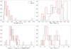 |
Fig. 8. Normalised histograms of the difference between the values obtained before and after subtraction of the ICL for the 19 candidate FGs (in red) and 30 non-FGs (in grey): effective radius (top left), absolute magnitude (top right), mean surface brightness (bottom left), and Sérsic index n (bottom right). |
Morphological parameters for FG and non-FG BGGs.
For non-FGs, the ICL increases the effective radius by a mean factor of 2.4 and the absolute magnitude with ICL is up to 1.2 mag brighter. The mean surface brightness before subtraction of the ICL can be up to 1.2 mag arcsec−2 fainter, with a mean of about 0.8, and the Sérsic index n tends to be larger with ICL, with a large dispersion from one BGG to another. We note that when the ICL is subtracted, the Sérsic index distributions become comparable for FGs and non-FGs (refer to Fig. 6). The distributions of the properties of BGGs obtained for FGs and non-FGs after ICL subtraction also become more comparable to those measured in the r filter (see Fig. 6). This is not surprising, as the r images before LSB processing should resemble rLSB images after the removal of low-brightness features. However, we also note that there is still a significant difference between the properties measured on the r and rLSB-ICL images. Indeed, BGGs on the r filter appear bigger, brighter, and have fainter mean surface brightnesses and higher Sérsic indices (see Table 3) than on rLSB-ICL images, all of which indicates the presence of ICL even on the r images. This illustrates the fact that ICL somewhat modifies the apparent morphological properties, and that its contribution should be carefully subtracted before analysing the physical properties of BCGs and BGGs.
4. Stellar populations of BGGs
4.1. Data
We retrieved the spectra of the FG and non-FG BGGs of our sample in the SDSS. Among the 87 FGs, 9 spectra were not available, leaving us with 78 BGGs. Among the 100 non-FGs, 4 spectra were not available, and so we analysed 96 spectra. We fit these spectra with Firefly (Wilkinson et al. 2017) and eliminated the spectra corresponding to AGN as classified by the SDSS: 13 in FGs and 14 in non-FGs. This was done because it is difficult to extract stellar populations from spectra dominated by an AGN. The AGN fractions are very similar between BGGs of FGs and non-FGs, namely 20% and 17%, respectively. We were therefore left with 66 FG BGG and 82 non-FG BGG spectra. As Wilkinson et al. (2017) showed that Kroupa and Salpeter IMFs gave comparable results, we limited our analysis to a Kroupa IMF. We used the STELIB and MILES stellar libraries to estimate the robustness of our results.
4.2. Results
We find that the stellar populations of FG and non-FG BGGs cannot be distinguished with this relatively straightforward analysis. As an illustration, we show the fraction of stellar mass created as a function of age in Fig. 9. Firefly fits the galaxy observed spectra using multiple star-formation bursts with various luminosities, masses, metallicities, and ages. The software returns the number of bursts, and for each burst gives its age, metallicity, and the fraction it contributed to the luminosity and stellar mass of the galaxy. From these, we computed the fraction of stellar mass formed in a range of galaxy age by summing the fractions of total stellar mass of all the star-formation bursts that occurred in the considered age range.
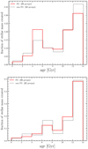 |
Fig. 9. Histograms of the fraction of stellar mass created as a function of age for FGs (red) and non-FGs (grey) for a Kroupa IMF using the MILES (top) and STELIB (bottom) libraries. |
We find that 76% and 71% of the total stellar mass of FG and non-FG BGGs, respectively, was already formed 8 Gyr ago based on the STELIB library. These percentages become 61% and 66% for the MILES library. These results agree with Fig. 5, where we see that the BGGs of FGs and non-FGs have very similar colours. Therefore, although the morphological properties of FG and non-FG BGGs somewhat differ, their stellar populations do not. Figure 9 shows that the choice between the MILES and STELIB libraries does not significantly affect the results.
There are 39 BGGs in FGs with emission lines (among which 9 may have a broad Hα component) out of 78. Each time Hα is detected, it is associated with the [NII]6584 emission line. For the BGGs of non-FGs, 30 out of 96 show emission lines (with no broad Hα line apparent).
These emission lines can originate from star-formation processes (e.g. driven by recent merging events) or from AGN activity (even if no broad Hα line is detected). However, the spectroscopy available to us comes from the SDSS survey, with a fiber of 3 arcsec diameter. Given the angular extent of the considered BGGs, at most 10% of their area within a Petrosian radius is covered by the fibre, and mainly in the centre of the galaxies. Detected emission lines are therefore probably coming from AGN activity, with rare cases where it can be produced by star-forming processes detected in the disk.
The respective percentages of Hα-[NII] emission line galaxies are 50% for FGs and 31% for non-FGs. This suggests that BGGs in FGs more frequently contain an AGN in their centre than those in non-FGs.
4.3. Emission lines in fossil-group BGGs: the case of NGC 4104
As seen in the previous section, a non-negligible fraction of our FG BGGs show emission lines and we think that these are mainly due to AGN activity. In order to more precisely investigate the location of the emitting regions in BGGs and see if some merging-induced star-formation activity can be detected, we concentrated on a specific example: NGC 4104 (not a member of our present sample of FG candidates). This is a well-known galaxy (see Fig. 10) at z ∼ 0.02816, and the BGG of the eponymous FG recently studied by Lima Neto et al. (2020), for example. It constitutes a good laboratory for investigating the possibility of having merging-induced star-formation activity because it is believed to have likely experienced relatively recent merging activity (Lima Neto et al. 2020). Given the fact that it is a nearby galaxy, it is also easy to study its spectral and morphological characteristics in detail.
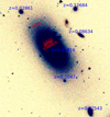 |
Fig. 10. SDSS g′, r′, i′ trichromic image (∼2.9′×3.5′) of NGC 4104. The redshifts indicated come from the SDSS. The red rectangles show the regions where we extracted MISTRAL spectra. |
Despite the BGG status of NGC 4104 (classified as S0 by the RC3 catalogue de Vaucouleurs et al. 1991, and as Elliptical by the SDSS), SDSS spectroscopy (identified as spec-2227-53820-0518 in the Science Archive Server) clearly shows strong emission lines in its centre (see Fig. 10 for the location of the SDSS spectroscopic extraction area). In this region, there is a noticeable lack of emission at the Hβ and [OIII] wavelengths. The Hα, [NII], and [SII] lines are very prominent, as are MgI and NaD absorption lines (see Fig. 11).
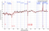 |
Fig. 11. SDSS spectroscopy of NGC 4104, with emission (blue labels) and absorption (red labels) lines. |
In order to investigate the origin of these emission lines, and to see whether or not they are present over the entire galaxy, we partially mapped NGC 4104 at the Observatoire de Haute-Provence with the MISTRAL single-slit spectro-imager4 in March 2022. We used the blue setting (one-hour exposure, resolution R ∼ 750, and covered the wavelength range [4200, 8000] Å) to obtain spectra in four different slits (see Fig. 10). The three slits close to the galaxy centre provided sufficiently high S/N to allow extraction of spectra in 15 different regions (see Fig. B.1). The outermost slit has insufficient S/N to detect any significant lines (including emission lines).
We do not detect any emission lines in the external regions of the galaxy with the other slits. Only central regions (l1, l2, l4, c1, c2, c3, c5, and c6 on Fig. B.1) show [NII], [SII], and sometimes weak-to-bright Hα emission, very similarly to what is visible in the SDSS spectrum. Figure B.1 shows a zoom onto the [6700, 6940] Å wavelength interval. The table GalSpecInfo of the SDSS DR17 database lists NGC 4104 as an AGN, with an old stellar population of the order of 13 Gyr. In order to investigate the nature of this galaxy more precisely, we first applied the pipes_vis visualisation tool (Leung et al. 2021) –which is based on the BAGPIPES tool (Carnall et al. 2018) – to the normalised SDSS spectrum. We selected a Wild et al. (2020) model, adding dust (Charlot & Fall 2000) and a nebular component (Leung et al. 2021).
First, based on Lima Neto et al. (2020), we assumed a stellar mass for NGC 4104 of 1011.3 M⊙ and a redshift of 0.03. We also fixed the α and β slopes of the Wild et al. (2020) burst (decline and incline steepness of the burst, index of double power law) to 100, the ηdust (additional scaling factor for dust in star forming clouds) to 2.0, the nCF00 (slope of the attenuation law) of the dust component to 0.7, and the tbc parameter in pipes_vis (time during which the star forming clouds remain) to 0.01 Gyr.
We then fixed the galaxy velocity dispersion to 150 km s−1 in order to reproduce the [SII] doublet aspect. The log(U) value (ionisation parameter) has to be lower than −3.5 in order to have [NII] stronger than Hα. We fixed log(U) to this value.
We had to introduce a passive population of older than ∼6 Gyr to explain the depth of the absorption lines. We fixed the age of the Universe when the older population formed to 8 Gyr. We also fixed the SFR decay timescale of the older population to 1 Gyr. To explain the absence of [OIII] emission and the weakness of Hβ, we fixed the metallicity to Z = 2.5 and the Av (extinction in V band) to 2. Finally, we added a small burst in the Wild et al. (2020) model, with 5% of the mass of the older population contained in the burst at ∼1 Gyr ago (12.8 Gyr after the Big Bang) in order to explain visible emission lines and to have sufficiently deep MgI and NaD lines. Values contained in the burst of more than 10% of the mass of the older population do not allow the spectrum characteristics to be reproduced, regardless of the values of the other parameters.
With this set of parameters, we are able to reasonably reproduce the SDSS spectrum (see Fig. 12). This probably shows that we are dealing with a relatively old stellar population (∼6 Gyr old). This is consistent with the 4–6 Gyr old merger proposed by Lima Neto et al. (2020). Any emission lines induced by the old merger have probably now vanished. In addition, a recent burst or merger (∼1 Gyr old) is also likely. It may possibly have reactivated the central AGN and be at the origin of the emission lines presently observed in the centre of NGC 4104. The star-forming Hα emission induced by this late merger event would require a few hundred million years to also vanish, and this is not in contradiction with the age of the recent burst (∼1 Gyr).
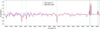 |
Fig. 12. Modelisation of the normalised SDSS spectrum of NGC 4104 with the pipes_vis tool. |
As a comparison to the other FGs, we also applied Firefly to the SDSS spectrum of NGC 4104 with a Kroupa IMF and the STELIB and MILES stellar libraries. For these two models, we find that 73% and 69% of the total stellar population was formed more than 8 Gyr ago, which is consistent with the previous results. The subtraction of the stellar population fitting results in a pure-emission spectrum that can be used to locate the line ratios in the BPT (Baldwin et al. 1981) diagrams (Kewley et al. 2013). The line ratios [OIII]/Hβ and [NII]/Hα locate the nuclear spectrum of NGC 4104 in the region occupied by LINER nuclei.
We also investigated the AGN nature of the spectra in the regions covered by MISTRAL where [NII] and Hα emissions are strong (namely regions c1, c2, and c5 of Fig. B.1). [OIII] and Hβ were not detectable, and so Fig. 13 only shows vertical lines for these three regions. We clearly see that, even without [OIII] and Hβ lines, the NGC 4104 c1, c2, c5, and central regions all have AGN characteristics.
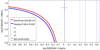 |
Fig. 13. log([OIII]5007/Hβ) versus log([NII]6584A/Hα) for the SDSS spectrum (central area, see e.g. Fig. B.1) and the c1, c2, and c5 MISTRAL regions. Regions under the red and blue curves are normal galaxies according to Kauffmann et al. (2003) and Kewley et al. (2013), respectively, while regions above these curves are active objects (AGN, LINERS). |
In conclusion, the emission lines of NGC 4104 originate mainly from the galaxy centre and each of the regions exhibiting emission lines have characteristics similar to those of AGN. The remaining areas of the galaxy have passive characteristics. The emission lines of NGC 4104 are therefore largely due to the AGN activity, in agreement with an AGN origin for the emission lines that we detected in at least part of our general sample of BGGs (see previous section).
5. Discussion and conclusions
The aim of this paper is to increase the number of known FGs to shed light on their formation process. Here, we increase the sample by adding 87 spectroscopically confirmed FG candidates with a high probability of being real FGs in view of their estimated large halo mass; though confirmation of the X-ray condition of their X-ray luminosity (LX > 1042 erg s−1) is still missing. For the FGs with UNIONS data available (35 in the u band, 25 in the r band and 19 in the rLSB band - r band treated with the Elixir-LSB software), we analysed the morphological properties of their BGG, and compared these properties with those of a control sample of 30 non-FG BGGs.
The 2D photometric fits of the BGGs made with GALFIT with one or two Sérsic components show that a single Sérsic component is sufficient in most objects in the u band, while two Sérsics are needed in the r band, both for FGs and non-FGs. However, non-FGs cover a larger range of Sérsic index n than FGs. Therefore, FG BGGs appear to have homogeneous profiles whereas non-FG BGGs cover a larger range of profiles.
After the subtraction of ICL in the rLSB images, the fraction of two-Sérsic BGGs increases. This is rather unexpected, because ICL forms a faint halo around the BGG and adds flux to the envelope of the BGG. We might therefore expect a higher fraction of two-Sérsic BGGs when ICL is included. However, the ICL distribution does not necessarily follow a Sérsic profile. In a more general way, it seems that Sérsic profiles do not trace physical components, and only act as an analytical description of galaxies.
FG BGGs appear to follow the Kormendy relation previously derived for BCGs by Chu et al. (2022), whereas the relation for non-FG BGGs is shifted to fainter surface brightnesses. This implies that FG BGGs have morphological properties that are more similar to those of BCGs, and may have evolved similarly to BCGs. Chu et al. (2021) confirmed that BCGs have not evolved since z = 1.8. Therefore, a similar evolution of FG BGGs and of BCGs favours the scenario in which FGs formed long ago and have since stopped evolving because their environment lacks galaxies that the group could otherwise have accreted.
We analysed the properties of the stellar populations of FG and non-FG BGGs derived from the analysis of their SDSS spectra with Firefly, assuming a Kroupa IMF and using the STELIB and MILES stellar libraries. We find no significant difference between FGs and non-FGs (65 and 82 galaxies respectively), and so the stellar populations of BGGs must have evolved in comparable ways in FGs and non-FGs.
Detailed observations of the FG NGC 4104 illustrate the fact that the BGGs of some FGs may show emission lines in their spectra. However, only a small percentage of BGGs are blue and star forming and could therefore potentially exhibit star-formation-induced Hα lines. The others, such as NGC 4104, show emission lines originating from their centre and mainly due to their AGN activity. In NGC 4104, this AGN was probably reactivated in the recent past by some merging activity, which puts the passive status of the central regions of FGs into question.
In conclusion, the BGGs of FGs and non-FGs are found to differ morphologically, suggesting they have followed somewhat different evolutionary pathways, but not sufficiently different to make their stellar populations distinguishable.
As a parallel project to increase the number of known FGs, we are presently obtaining spectroscopic confirmation of the subsample of FG candidates detected in the CFHTLS survey with a high probability by Adami et al. (2020). This will be the topic of a future paper.
Acknowledgments
We thank the referee, Rémi Cabanac, for his careful and constructive reading of the manuscript. We are grateful to Nicolas Clerc for matching our FG and non-FG catalogues with his XCLASS X-ray catalogue. F.D. acknowledges support from CNES. I.M. acknowledges financial support from the State Agency for Research of the Spanish MCIU, through the “Center of Excellence Severo Ochoa” award to the Instituto de Astrofísica de Andalucía (SEV-2017-0709), and through PID2019-106027GB-C41. F.S. acknowledges support from a CNES Postdoctoral Fellowship. This work is based on data obtained as part of UNIONS (initially CFIS), using data from a CFHT large program of the National Research Council of Canada and the French Centre National de la Recherche Scientifique. Based on observations obtained with MegaPrime/MegaCam, a joint project of CFHT and CEA Saclay, at the Canada-France-Hawaii Telescope (CFHT) which is operated by the National Research Council (NRC) of Canada, the Institut National des Science de l’Univers (INSU) of the Centre National de la Recherche Scientifique (CNRS) of France, and the University of Hawaii. Pan-STARRS is a project of the Institute for Astronomy of the University of Hawaii, and is supported by the NASA SSO Near Earth Observation Program under grants 80NSSC18K0971, NNX14AM74G, NNX12AR65G, NNX13AQ47G, NNX08AR22G, and by the State of Hawaii. Funding for the Sloan Digital Sky Survey IV has been provided by the Alfred P. Sloan Foundation, the U.S. Department of Energy Office of Science, and the Participating Institutions. SDSS-IV acknowledges support and resources from the Center for High-Performance Computing at the University of Utah. The SDSS web site is www.sdss.org. SDSS-IV is managed by the Astrophysical Research Consortium for the Participating Institutions of the SDSS Collaboration including the Brazilian Participation Group, the Carnegie Institution for Science, Carnegie Mellon University, the Chilean Participation Group, the French Participation Group, Harvard-Smithsonian Center for Astrophysics. Based in part on observations made at Observatoire de Haute-Provence (CNRS), France. This research has made use of the MISTRAL database, based on observations made at Observatoire de Haute Provence (CNRS), France, with the MISTRAL spectro-imager, and operated at CeSAM (LAM), Marseille, France. Based on observations collected at Centro Astronomico Hispano en Andalucia (CAHA) at Calar Alto, operated jointly by Instituto de Astrofisica de Andalucia (CSIC) and Junta de Andalucia. Based on observations taken with the Nordic Optical Telescope on La Palma (Spain).
References
- Adami, C., Giles, P., Koulouridis, E., et al. 2018, A&A, 620, A5 [NASA ADS] [CrossRef] [EDP Sciences] [Google Scholar]
- Adami, C., Sarron, F., Martinet, N., & Durret, F. 2020, A&A, 639, A97 [NASA ADS] [CrossRef] [EDP Sciences] [Google Scholar]
- Aguerri, J. A. L., & Zarattini, S. 2021, Universe, 7, 132 [NASA ADS] [CrossRef] [Google Scholar]
- Baldwin, J. A., Phillips, M. M., & Terlevich, R. 1981, PASP, 93, 5 [Google Scholar]
- Bertin, E. 2006, in Astronomical Data Analysis Software and Systems XV, eds. C. Gabriel, C. Arviset, D. Ponz, & S. Enrique, ASP Conf. Ser., 351, 112 [Google Scholar]
- Bertin, E., & Arnouts, S. 1996, A&AS, 117, 393 [NASA ADS] [CrossRef] [EDP Sciences] [Google Scholar]
- Bertin, E., Mellier, Y., Radovich, M., et al. 2002, in Astronomical Data Analysis Software and Systems XI, eds. D. A. Bohlender, D. Durand, & T. H. Handley, ASP Conf. Ser., 281, 228 [NASA ADS] [Google Scholar]
- Bharadwaj, V., Reiprich, T. H., Sanders, J. S., & Schellenberger, G. 2016, A&A, 585, A125 [NASA ADS] [CrossRef] [EDP Sciences] [Google Scholar]
- Campbell, D., van den Bosch, F. C., Hearin, A., et al. 2015, MNRAS, 452, 444 [NASA ADS] [CrossRef] [Google Scholar]
- Cao, J.-Z., Tinker, J. L., Mao, Y.-Y., & Wechsler, R. H. 2020, MNRAS, 498, 5080 [NASA ADS] [CrossRef] [Google Scholar]
- Carnall, A. C., McLure, R. J., Dunlop, J. S., & Davé, R. 2018, MNRAS, 480, 4379 [Google Scholar]
- Charlot, S., & Fall, S. M. 2000, ApJ, 539, 718 [Google Scholar]
- Chen, Y.-M., Kauffmann, G., Tremonti, C. A., et al. 2012, MNRAS, 421, 314 [NASA ADS] [Google Scholar]
- Chu, A., Durret, F., & Márquez, I. 2021, A&A, 649, A42 [NASA ADS] [CrossRef] [EDP Sciences] [Google Scholar]
- Chu, A., Sarron, F., Durret, F., & Márquez, I. 2022, A&A, 666, A54 [NASA ADS] [CrossRef] [EDP Sciences] [Google Scholar]
- Dariush, A., Khosroshahi, H. G., Ponman, T. J., et al. 2007, MNRAS, 382, 433 [NASA ADS] [CrossRef] [Google Scholar]
- de Vaucouleurs, G., de Vaucouleurs, A., Corwin, H. G. J., et al. 1991, S&T, 82, 621 [NASA ADS] [Google Scholar]
- D’Onghia, E., Sommer-Larsen, J., Romeo, A. D., et al. 2005, ApJ, 630, L109 [CrossRef] [Google Scholar]
- Duc, P.-A., Cuillandre, J.-C., Karabal, E., et al. 2015, MNRAS, 446, 120 [Google Scholar]
- Ellien, A., Slezak, E., Martinet, N., et al. 2021, A&A, 649, A38 [NASA ADS] [CrossRef] [EDP Sciences] [Google Scholar]
- Ferrarese, L., Côté, P., Cuillandre, J.-C., et al. 2012, ApJS, 200, 4 [Google Scholar]
- Fukugita, M., Shimasaku, K., & Ichikawa, T. 1995, PASP, 107, 945 [Google Scholar]
- Girardi, M., Aguerri, J. A. L., De Grandi, S., et al. 2014, A&A, 565, A115 [NASA ADS] [CrossRef] [EDP Sciences] [Google Scholar]
- Ilbert, O., Arnouts, S., McCracken, H. J., et al. 2006, A&A, 457, 841 [NASA ADS] [CrossRef] [EDP Sciences] [Google Scholar]
- Jiménez-Teja, Y., Dupke, R., Benítez, N., et al. 2018, ApJ, 857, 79 [Google Scholar]
- Jones, L. R., Ponman, T. J., Horton, A., et al. 2003, MNRAS, 343, 627 [NASA ADS] [CrossRef] [Google Scholar]
- Kauffmann, G., Heckman, T. M., Tremonti, C., et al. 2003, MNRAS, 346, 1055 [Google Scholar]
- Kewley, L. J., Maier, C., Yabe, K., et al. 2013, ApJ, 774, L10 [Google Scholar]
- Kim, D.-W., Anderson, C., Burke, D., et al. 2018, ApJ, 853, 129 [NASA ADS] [CrossRef] [Google Scholar]
- Kormendy, J. 1977, ApJ, 218, 333 [NASA ADS] [CrossRef] [Google Scholar]
- La Barbera, F., de Carvalho, R. R., de la Rosa, I. G., et al. 2009, AJ, 137, 3942 [NASA ADS] [CrossRef] [Google Scholar]
- Leung, H.-H., Wild, V., Carnall, A., & Papathomas, M. 2021, Res. Notes Am. Astron. Soc., 5, 171 [Google Scholar]
- Lima Neto, G. B., Durret, F., Laganá, T. F., et al. 2020, A&A, 641, A95 [NASA ADS] [CrossRef] [EDP Sciences] [Google Scholar]
- Margalef-Bentabol, B., Conselice, C. J., Mortlock, A., et al. 2016, MNRAS, 461, 2728 [Google Scholar]
- Peng, C. Y., Ho, L. C., Impey, C. D., & Rix, H.-W. 2002, AJ, 124, 266 [Google Scholar]
- Ponman, T. J., Allan, D. J., Jones, L. R., et al. 1994, Nature, 369, 462 [Google Scholar]
- Romer, A. K., Nichol, R. C., Holden, B. P., et al. 2000, ApJS, 126, 209 [NASA ADS] [CrossRef] [Google Scholar]
- Santos, W. A., Mendes de Oliveira, C., & Sodré, L. Jr. 2007, AJ, 134, 1551 [NASA ADS] [CrossRef] [Google Scholar]
- Sarron, F., Martinet, N., Durret, F., & Adami, C. 2018, A&A, 613, A67 [NASA ADS] [CrossRef] [EDP Sciences] [Google Scholar]
- Tinker, J., Wetzel, A., & Conroy, C. 2011, ArXiv eprints [arXiv:1107.5046] [Google Scholar]
- Tinker, J. L. 2021, ApJ, 923, 154 [NASA ADS] [CrossRef] [Google Scholar]
- Vikhlinin, A., McNamara, B. R., Hornstrup, A., et al. 1999, ApJ, 520, L1 [NASA ADS] [CrossRef] [Google Scholar]
- von Benda-Beckmann, A. M., D’Onghia, E., Gottlöber, S., et al. 2008, MNRAS, 386, 2345 [NASA ADS] [CrossRef] [Google Scholar]
- Žemaitis, R., Ferguson, A. M. N., Okamoto, S., et al. 2023, MNRAS, 518, 2497 [Google Scholar]
- Wild, V., Taj Aldeen, L., Carnall, A., et al. 2020, MNRAS, 494, 529 [NASA ADS] [CrossRef] [Google Scholar]
- Wilkinson, D. M., Maraston, C., Goddard, D., Thomas, D., & Parikh, T. 2017, MNRAS, 472, 4297 [Google Scholar]
- Yang, X., Mo, H. J., van den Bosch, F. C., & Jing, Y. P. 2005, MNRAS, 356, 1293 [Google Scholar]
- Zarattini, S., Aguerri, J. A. L., Calvi, R., & Girardi, M. 2022, A&A, 668, A38 [NASA ADS] [CrossRef] [EDP Sciences] [Google Scholar]
Appendix A: Lists of FG candidates and non-FGs
The list of the 87 FG candidates is given in Table A.1 with the principal properties of their BGG. The list of the 30 non-FGs for which the morphological properties were analysed here is shown in Table A.2. The full list of 100 non-FGs will be made available in electronic form at the CDS, together with the list of 87 FG candidates.
Sample of 87 FG candidates.
Control sample of 30 non-FG candidates.
Appendix B: Spectra of NGC 4104
Illustrations of the observations obtained with the MISTRAL spectrograph at Observatoire de Haute Provence are given in Fig. B.1.
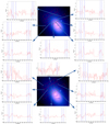 |
Fig. B.1. MISTRAL spectroscopic observations of 15 different regions of NGC 4104. Spectra are normalised in flux. The location of the SDSS fibre is shown as the blue central circle. The wavelength domain is limited to [6700, 6940]Å. |
All Tables
All Figures
|
Fig. 1. Normalised histograms of the logarithms of the halo masses for FGs (red) and non-FGs (grey). Top: 87 FGs and 100 non-FGs. Bottom: 25 FGs and 30 non-FGs analysed morphologically. |
| In the text | |
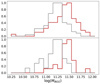 |
Fig. 2. Same as Fig. 1 for the normalised histograms of the logarithms of the BGG stellar masses. |
| In the text | |
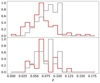 |
Fig. 3. Same as Fig. 1 for the normalised redshift histograms. |
| In the text | |
|
Fig. 4. Normalised histograms of the absolute magnitudes of the BGGs in the g (top) and r (middle) bands, and of the (g − r) colour (bottom) for FGs (red) and non-FGs (grey). Left: 87 FGs and 100 non-FGs. Right: 25 FGs and 30 non-FGs analysed morphologically. |
| In the text | |
|
Fig. 5. (g − r) colour magnitude diagram for four samples: light red dots: galaxies within 1 arcmin of FG BGGs; red stars: FG BGGs; grey dots: all galaxies within 1 arcmin of non-FG BGGs; black stars: non-FG BGGs. The x-axis is the absolute magnitude in the r band. A zoomed-in version of the plot at the brightest magnitudes is shown in the top right corner. |
| In the text | |
|
Fig. 6. Normalised histograms of the effective radius, absolute magnitude, mean surface brightness corrected for cosmological dimming, and Sérsic index n (from left to right). From top to bottom: 35 candidate FGs (in blue) and 30 non-FGs (grey) in the u band; 25 candidate FGs (in red) and 30 non-FGs (grey) in the r band; 19 candidate FGs (green) and 30 non-FGs (grey) in the rLSB band; same as above in the rLSB band after ICL subtraction (yellow for FGs). |
| In the text | |
|
Fig. 7. Kormendy relation for FGs in red and non-FGs in grey, superimposed on the relation found for almost 1000 BCGs by Chu et al. (2022) in cyan. Both plots are obtained in the rLSB band, the top plot without ICL subtraction and the bottom plot after ICL subtraction. The points for FGs and non-FGs have been shifted from the r to the i band, and all points are corrected for cosmological dimming. |
| In the text | |
|
Fig. 8. Normalised histograms of the difference between the values obtained before and after subtraction of the ICL for the 19 candidate FGs (in red) and 30 non-FGs (in grey): effective radius (top left), absolute magnitude (top right), mean surface brightness (bottom left), and Sérsic index n (bottom right). |
| In the text | |
|
Fig. 9. Histograms of the fraction of stellar mass created as a function of age for FGs (red) and non-FGs (grey) for a Kroupa IMF using the MILES (top) and STELIB (bottom) libraries. |
| In the text | |
|
Fig. 10. SDSS g′, r′, i′ trichromic image (∼2.9′×3.5′) of NGC 4104. The redshifts indicated come from the SDSS. The red rectangles show the regions where we extracted MISTRAL spectra. |
| In the text | |
|
Fig. 11. SDSS spectroscopy of NGC 4104, with emission (blue labels) and absorption (red labels) lines. |
| In the text | |
|
Fig. 12. Modelisation of the normalised SDSS spectrum of NGC 4104 with the pipes_vis tool. |
| In the text | |
|
Fig. 13. log([OIII]5007/Hβ) versus log([NII]6584A/Hα) for the SDSS spectrum (central area, see e.g. Fig. B.1) and the c1, c2, and c5 MISTRAL regions. Regions under the red and blue curves are normal galaxies according to Kauffmann et al. (2003) and Kewley et al. (2013), respectively, while regions above these curves are active objects (AGN, LINERS). |
| In the text | |
|
Fig. B.1. MISTRAL spectroscopic observations of 15 different regions of NGC 4104. Spectra are normalised in flux. The location of the SDSS fibre is shown as the blue central circle. The wavelength domain is limited to [6700, 6940]Å. |
| In the text | |
Current usage metrics show cumulative count of Article Views (full-text article views including HTML views, PDF and ePub downloads, according to the available data) and Abstracts Views on Vision4Press platform.
Data correspond to usage on the plateform after 2015. The current usage metrics is available 48-96 hours after online publication and is updated daily on week days.
Initial download of the metrics may take a while.