| Issue |
A&A
Volume 682, February 2024
|
|
|---|---|---|
| Article Number | A86 | |
| Number of page(s) | 21 | |
| Section | Stellar atmospheres | |
| DOI | https://doi.org/10.1051/0004-6361/202345919 | |
| Published online | 08 February 2024 | |
Stellar activity and differential rotation of HD 111395
1
Hamburger Sternwarte, Universität Hamburg,
Gojenbergsweg 112,
21029
Hamburg,
Germany
e-mail: mmittag@hs.uni-hamburg.de
2
Departamento de Astronomia, Universidad de Guanajuato,
Callejón de Jalisco s/n,
36023
Guanajuato,
GTO,
Mexico
Received:
17
January
2023
Accepted:
31
October
2023
Aims. Stellar activity cycles and rotation periods are important parameters for characterising the stellar dynamo, which operates in late-type main-sequence stars. However, the number of stars with well-known cycle and rotation periods is rather low, so new detections are still important.
Methods. To find activity cycles and rotation periods, we utilised the TIGRE telescope to monitor stars for periodic variations in chromospheric activity indicators. We employed the widely used CaII H&K lines and the CaII infrared triplet lines as stellar activity indicators. To verify a periodic variation and to determine the corresponding period, we performed a frequency analysis via the generalised Lomb-Scargle method of the taken time series.
Results. We studied CaII data of the G5V star HD 111395 and derive an activity cycle period of 949 ± 5 d (≈2.6 yr). This cycle is coincident with coronal measurements from the X-ray telescope eROSITA on board SRG. Furthermore, the TIGRE CaII time series show a long-term trend that indicates an additional long-term cycle. Using the few available literature S-index data points, we estimate a probable cycle length of 12–15 yr for this potential long-term cycle. Finally, we determined rotation periods from each observation season. We computed a mean rotation period of 16.76 ± 0.36 d averaged over all observation seasons and chromospheric indicators. However, we also find a strong variation in the mean seasonal rotation periods, which follows the derived cycle period; therefore, we interpret this behaviour as a sign of surface differential rotation.
Key words: stars: activity / stars: chromospheres / stars: coronae / stars: late-type / stars: rotation / X-rays: stars
© The Authors 2024
 Open Access article, published by EDP Sciences, under the terms of the Creative Commons Attribution License (https://creativecommons.org/licenses/by/4.0), which permits unrestricted use, distribution, and reproduction in any medium, provided the original work is properly cited.
This article is published in open access under the Subscribe to Open model. Subscribe to A&A to support open access publication.
1 Introduction
With the term ‘stellar activity’, one typically summarises all phenomena related to non-radiative heating in the outer layers of late-type stars. These ‘activity’ phenomena are connected with magnetic fields, which are thought to be created by a stellar dynamo, usually assumed to be the so-called α − Ω dynamo introduced by Parker (1955). Thus, by studying the phenomena created by the magnetic field, one also have the possibility to study the stellar dynamo.
The most obvious phenomena of solar magnetic activity are sunspots, which are directly observable, at some rare times even without a telescope. However, the systematic recording of sunspots started only at the beginning of the 17th century, after the invention of the telescope by Galileo. The sunspots are seen to move over the solar disk, which allowed Galileo to determine the rotation period of the Sun; furthermore, the number of sunspots visible on the solar disk at any given time shows a long-term periodic variation with a period of 11 yr, which was first recognised by Schwabe (1844).
Stars cannot be spatially resolved, and thus other means are required to study the stellar analogues of solar activity. Eberhard & Schwarzschild (1913) discovered that the Ca II H&K lines are sensitive to stellar activity, and much later O. C. Wilson used this finding for a systematic monitoring of stars to detect activity cycles and to determine the corresponding cycle length, starting in 1966 (Wilson 1978). For this monitoring, an instrumental Ca II H&K index was introduced (which we refer to here as the Mount Wilson S-index), which characterises the chromospheric activity of a star. The Mount Wilson programme ran for more than three decades; a final outcome was presented in the landmark paper by Baliunas et al. (1995), where the time series of 112 stars (including the Sun) are presented together with a search for stellar cycles in this sample. With the release of the Mount Wilson S-index database1, a re-analysis of all of the Mount Wilson S-index data became possible (see e.g. Boro Saikia et al. 2018; Olspert et al. 2018).
After the termination of the Mount Wilson programme, some successor observation programmes were carried out, for example the Solar-Stellar Spectrograph (SSS) programme at the Lowell Observatory (Hall et al. 2007; Radick et al. 2018), the SMARTS (Small & Moderate Aperture Research Telescope System) southern HK project by Metcalfe et al. (2010), 2013), and a number of long-term stellar activity monitoring programmes with the TIGRE (Telescopio Internacional de Guanajuato Robótico Espectroscópico) telescope (e.g. Mittag et al. 2019; Schröder et al. 2020). Furthermore, the spectra taken in the context of some radial-velocity monitoring programmes to detect extrasolar planets often cover the Ca II H&K lines, so these data can also be used to determine Mount Wilson S-indices and study stellar activity phenomena. Such programmes are carried out for example with HIRES (High Resolution Echelle Spectrometer) and the HARPS (High Accuracy Radial velocity Planet Searcher) spectrograph. The California Planet Search (CPS) was performed with HIRES, and, based on these data, S-index values were determined and published by Wright et al. (2004) and Isaacson & Fischer (2010). In Baum et al. (2022), the combined time series of the Mount Wilson S-index data and the HIRES S-index data for 59 stars have been published and the results of a time series analysis presented. Boro Saikia et al. (2018) studied the chromospheric activity of 4454 cool stars from a collection of chromospheric activity data from different data sources, re-determined the cycle periods of 39 Mount Wilson stars, and determined new cycle periods for 14 stars based on HARPS data.
Chromospheric activity indices based on chromospheric lines are not the only way to find activity cycles. They can also be detected via photometry (Suárez Mascareño et al. 2016) and, for a few stars, via X-ray measurements (see e.g. detections for single stars by Robrade et al. 2012; Wargelin et al. 2017).
In addition to the cycle determinations, the measurement of the rotation period of a star is an essential task in the field of stellar activity. Rotation lies at the core of all stellar activity indicators of late-type stars. Unfortunately, rotation measurements are not that straightforward (see the discussion by Schmitt & Mittag 2020), in particular for stars with lower activity levels. Furthermore, the activity cycle period and the rotation period are correlated, as first found by Noyes et al. (1984), which let these authors use the Rossby number instead the rotation period. Tuominen et al. (1988) showed that the cycle-rotation connection is described theoretically by the relation  , where Pcyc is the cycle period, Prot the rotation period, and dConv the fractional depth of the convection zone. Later and more extensive studies, such as those by Saar & Baliunas (1992), actually found two cycle branches, usually denoted as ‘active’ and ‘inactive’ branches, and Böhm-Vitense (2007) showed that the slopes in the relation between the activity cycle period and rotation period are similar for the two branches. In this cycle period-rotation period presentation, the 11-yr solar cycle is located in between these two branches, raising the question of whether the solar cycle is a special case. To explain this unusual position, Böhm-Vitense (2007) speculated that the solar cycle is influenced by different dynamo types. Another approach to explaining the solar cycle position has been put forward by Metcalfe et al. (2016), who assumed the solar dynamo to be in a transitional evolutionary phase. Furthermore, the Sun is not the only star where a transitional dynamo may be at work (see Metcalfe et al. 2016, 2022; Metcalfe & van Saders 2017). However, Boro Saikia et al. (2018) also studied the cycle–rotation connection, taking into consideration the 14 possible cycles determined from the HARPS data, and concluded that the Sun is likely not in such a transitional evolutionary phase.
Brandenburg et al. (2017) present a detailed study of the cycle–rotation connection using data from different sources. They separated the data into two samples, one containing type F and G stars and one containing type K stars. They proceeded to derive relations between the ratios ωcyc/Ω = Prot/Pcyc and the activity index R′HK for the two (sub-)samples as well as for the two cycle branches. With this split into different B-V ranges, they assumed a dependence on stellar mass, or rather effective temperature, in the cycle–rotation connection. However, the fit parameter of the derived relations is comparable for both (sub-)samples, except for the exponent of R′HK for the long-cycle branch (see Brandenburg et al. 2017, Table 1). This indicates that the relation by Brandenburg et al. (2017) is independent of stellar mass, or rather the effective temperature!
Mittag et al. (2023) re-analysed the cycle period–rotation period connection using the Rossby number instead of the rotation period. In the cycle–Rossby number presentation, a clear split into different B – V ranges is observable, which indicates a dependence on stellar mass, or rather the effective temperature (see also Sect. 6.1). Furthermore, in the cycle–Rossby number presentation, the solar cycle follows the general trend and there is no need to introduce a special transitional evolutionary phase.
The total number of stars with well-known activity cycles and rotation periods is very limited (fewer than 50 stars), and currently the best collections of these stars are those from Brandenburg et al. (2017) and Mittag et al. (2023). Due to these numerical limitations, the search for such stars remains an important undertaking.
In the context of dynamo theory, it is actually the differential rotation that matters. It is responsible for magnetic field production, and, not surprisingly, the measurement of differential rotation is even more difficult than the measurement of a single rotation period or an activity cycle.
For the Sun, differential rotation is readily established by following the motion of sunspots as a function of the appearance latitude, ϕ. According to Newton & Nunn (1951), the solar differential rotation is described by the rotation law Ω(ϕ) = 14.38 − 2.44 sin2(ϕ) (in deg/day), where Ω(ϕ) is the latitude-dependent rotation rate. Furthermore, if one considers the appearance latitudes of sunspots as a function of cycle phase, a so-called butterfly diagram is observed, since sunspots tend to appear at higher latitudes (both northern and southern) at the beginning of a cycle at around 30°, while at the end of the cycle they appear much closer to the solar equator, hence producing the appearance of butterfly wings.
Clearly, in the case of a star a butterfly diagram cannot be observed directly. Nevertheless, the rotational signal in a photometric or S-index time series is often produced by just a few, unevenly active regions in the dominant latitude. The rotational signal can be expected to vary with any latitudinal changes in the active regions and, therefore, with the cycle phase (see also Sect. 5.6.1).
A landmark study in the field of differential rotation periods is the paper by Donahue et al. (1996), who presented the variation in the rotation period caused by surface differential rotation for a sample of stars. Donahue et al. (1996) found a correlation between the maximal and minimal values of the rotation period and the mean rotation period. Reinhold et al. (2013) used Kepler data to determine differential rotation rates and showed that they increase with rotation. A critical discussion of the possibility of measuring differential rotation based on broadband precision light curves is presented by Basri & Shah (2020), who conclude that such measurements are only possible if the spot lifetimes are much longer than the rotation period of the star.
The TIGRE stellar activity monitoring programme is being carried out to verify already known activity cycles and find new ones (see e.g. Mittag et al. 2019). In this paper, we present the results of our observations of HD 111395. We show time series of S-indices based on the Ca II H&K and infrared triplet (IRT) lines and present the results of our cycle search. We then study the time series to find a rotational modulation in our Ca II data. Finally, we discuss the clear variation in the seasonal rotation periods and interpret them in terms of differential rotation.
2 Stellar parameters of HD 111395
HD 111395 (also known as GJ 486.1) is a nearby star with a parallax of 58.486 ± 0.029 mas from Gaia Collaboration (2022) (which leads to a distance of d = 17.098 ± 0.009 pc). It is therefore quite bright (mV = 6.29 mag) with a colour index B − V of 0.703 mag (ESA 1997); in the SIMBAD database it is listed as a G5 main-sequence star and classified as a variable of the BY Dra type. The PASTEL catalogue by Soubiran et al. (2016), version 2020-01-30) lists various values of the stellar parameters Teff, log(ɡ) and [Fe/H]. Hence, we computed the median for the stellar parameters and assumed the computed standard deviation as uncertainty for these values and listed these results in Table 1. The Gaia Data Release 2 catalogue (Gaia Collaboration 2018) lists a bolometric luminosity for HD 111395 (see Table 1), which we used for our log(LX/Lbol) value value of HD 111395 (see Sect. 4.3).
A mean rotational velocity (υsin(i)) of HD 111395 is given with 2.8 km/s in the Głębocki & Gnaciński (2005) catalogue. Strassmeier et al. (1999) determined a rotation period of 15.8 days based on photometry, the rotation period was also measured based on Ca II H&K and IRT data by Mittag et al. (2017a), resulting in a value of 16.2 ± 0.1 d; both values are consistent with each other.
Stellar parameters of HD 111395.
3 TIGRE observations of HD 111395
Using the robotic TIGRE telescope located at the La Luz Observatory in central Mexico, we have regularly monitored HD 111395 since 2014, when TIGRE started its robotic operations. TIGRE is equipped with the two channel fibre-fed Échelle spectrograph HEROS (Heidelberg Extended Range Optical Spectrograph), which covers the wavelength range from 3738 Å to 8838 Å with a small gap around 5750 Å. The average spectral resolution in both spectral channels is ≈20 000, and a detailed description of the TIGRE telescope and its operations has been provided by Schmitt et al. (2014) and González-Pérez et al. (2022).
The recorded spectra are reduced with the TIGRE standard fully automatic reduction pipeline v3.1, described by Mittag et al. (2010, 2016); Hempelmann et al. (2016). The pipeline includes an automatic determination of the activity index based on the Ca II H&K lines, the so-called TIGRE S-index. It is defined as the ratio of the line area in a 1Å rectangular band pass centred on the Ca II H&K lines and two 20 Å wide quasi-continua centred at 3901.07 Å and 4001.07 Å (Mittag et al. 2016). To compare our TIGRE S-index measurement based on the Ca II H&K lines with measurements taken with other instruments, the STIGRE index is converted into the most common activity scale, the Mount Wilson S-index, using the equation derived by Mittag et al. (2016):
 (1)
(1)
The TIGRE spectra also include the Ca II IRT lines at 8498 Å, 8542 Å, and 8662 Å; these lines are also sensitive to stellar activity and are strongly correlated with the Ca II H&K lines (Martin et al. 2017; Mittag et al. 2017a). Mittag et al. (2017a) define activity indices based on the Ca II IRT lines, denoted as SIRT_8498, SIRT_8542, and SIRT_8662, respectively; as with the TIGRE S-index, these indices are determined automatically during the pipeline data reduction.
For HD 111395, we collected a total of 349 SMWO values and 311 SIRT values for each of the Ca II IRT lines, and in Table 2 we list the total number of S-values taken in each observation season, the corresponding seasonal mean S-value and the standard deviation of these S-values. The reason for the difference between the total numbers of the S MWO and IRT S-values was a technical problem with the CCD for the red spectral channel of HEROS: from November 2014 to May 2015, the red CCD camera was defect and replaced by a spare CCD camera, which had a rather strong memory effect. To avoid any ambiguities, we therefore decided not to use those red spectra.
4 Stellar activity of HD 111395
Before presenting our TIGRE observations in detail, we present a general overview of the stellar activity of HD 111395. The signal in the different wavelength ranges is formed in different atmospheric layers, so we can detect and study the stellar activity in the different atmospheric layers. First, we consider the photometric data formed in the photosphere of the star. Then, we discuss Ca II data, including our new TIGRE data, which reveal the stellar activity in the chromospheric layer, and finally, we analyse the available X-ray data of HD 111395 to investigate its coronal activity.
4.1 Photosphere
Variability of the photometric light curve is a typical signature of star spots and hence stellar activity. To investigate the short-term photometric variability, we used the available public TESS (Transiting Exoplanet Survey Satellite) data.
The TESS mission provides photometric light curves (Ricker et al. 2015) for large numbers of stars simultaneously. TESS’s four cameras observe a field of view of 24° × 96° more or less continuously for 27 days; then the viewing direction is changed and another sky region is observed. The recorded data are publicly available, for example via the MAST (Mikulski Archive for Space Telescopes) portal2. The TESS light curves are available with two fluxes, the SAP (Simple Aperture Photometry) flux [e− s−1] and the PDCSAP (Pre-search Data Conditioning SAP) flux [e− s−1]. The PDCSAP flux is a corrected SAP flux (Stumpe et al. 2012; Smith et al. 2012) in which instrumental variations are taken into consideration; the timescale used in the TESS light curve is given as a barycentric TESS Julian date (BTJD), which is defined as BTJD = BJD − 2 457 000.0 days.
HD 111395 was observed in 2020 and in 2022 with TESS. We show the available TESS SAP light curves in Fig. 1, where we normalised the SAP flux with the mean flux in the corresponding time range. In both datasets, a clear flux variation in the time range 15 to 20 days is visible, which is very likely caused by stellar rotation, especially when the results of the Ca II data are taken into account, as discussed later in Sect. 5.
The determination of the rotation period based on these TESS data is problematic due to the length of the expected rotation period and the length of the time series because only one complete rotation cycle is observable; furthermore, the time series may contain also instrumental variations. At this point, we want to mention that the PDCSAP light curve for the 2022 does not show the 20 day variation. Here, we assumed that the correction of the SAP flux probably failed for this light curve; therefore, we only show the two SAP light curves.
In Fig. 1, the peak-to-peak variations amount to ≈ 1%, indicating strong photometric variability and magnetic activity; for comparison, our Sun shows a variability of ≈0.12% in the total solar irradiance between the activity minimum and maximum (e.g. Kopp & Lean 2011). Thus, the photometric variability of HD 111395 is a factor of 8 larger. However, we need to keep in mind that the peak-to-peak variations of HD 111395 show the variation caused by the stellar rotation and that these variations are usually smaller than the variation between the activity minimum and maximum. Therefore, one can assume that the variability of HD 111395 is even larger than this factor of 8.
We conclude that, in this case, the TESS light curves are too short to allow us to determine a reliable rotation period. However, the TESS light curves confirm that HD 111395 is a spotted star, which merits further photometric observations.
Furthermore, we additionally retrieved photometric light curves from the HIPPARCOS catalogue (ESA 1997) and the All Sky Automated Survey (ASAS) data, presented by Pojmanski (1997) and published in the ASAS-3 photometric V-band catalogue3 (taken from 2003 to 2009). However, the errors in both datasets are too large and/or data sampling to sparse to see the photometric short-term variability found in the TESS data.
Information on the different seasonal mean S-values.
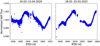 |
Fig. 1 Normalised TESS light curves. The left panel shows the light curve taken in 2020 from March 20 to April 15, and the right panel shows the light curve taken in 2022 from February 26 to March 25. |
Mean S-values, standard deviation (σS –value), and the relative scatter.
4.2 Chromosphere
The most common indicator for the chromospheric activity is the Mount Wilson S-index (SMWO; Wilson 1978; Baliunas et al. 1995; Vaughan et al. 1978), but unfortunately HD 111395 was not part of the Mount Wilson programme. However, it was observed in other stellar activity surveys where SMWO-values were estimated. We found S-values by Gray et al. (2003) with SMWO = 0.227, Wright et al. (2004) with SMWO = 0.290 and Isaacson & Fischer (2010) with a median SMWO = 0.306. For comparison, we computed the mean S-value for the Ca II H&K and IRT lines taken from our TIGRE time series, the corresponding standard deviation (σS –value) and a relative scatter (σS –value/mean S-value) of our S-values. These results are listed in Table 3. The computed mean TIGRE SMWO value is consistent with previously reported S-values.
The SMWO values range from 0.227 to 0.306, suggesting a high level and strong variations in chromospheric activity. Based on our mean SMWO, we calculated the activity index  , which is the pure Ca II flux excess (Mittag et al. 2013). Using the effective temperature, Teff, of 5589 K, computed with the Teff(B − V) relation from Gray (2005, Eq. (14.17)), we obtain a log
  value of −4.47 for HD 111395.
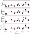 |
Fig. 2 Time series of the Ca II activity indices. From top to bottom, the SMWO, SIRT_8498, SIRT_8542, and SIRT_8662 time series are plotted (black dots). The dashed red line in each panel represents the best-fit linear trend. |
4.3 Corona
X-ray emission in main-sequence stars is a clear proxy indicator for stellar magnetic activity. In the ROSAT (Roentgen Satellite) all-sky survey HD 111395 was detected as a rather strong X-ray source with a count rate of 0.133 ± 0.021 counts s−1, corresponding to an X-ray luminosity LX = 2.5 1028 erg s−1 Hünsch et al. (1999), which leads to a (logarithmic) LX/Lbol -ratio of −5.11, indicating a moderately active corona. In the more recent eROSITA (extended Roentgen Survey with an Imaging Telescope Array) all-sky survey (Predehl et al. 2021), HD 111395 was also detected as an X-ray source, and Fuhrmeister et al. (2022) derive a log(LX/Lbol) value of −5.137 ± 0.050, consistent with the earlier ROSAT results.
5 Variability in the Ca II H&K and IRT lines
5.1 Overview
In this section, we discuss our results of the TIGRE observations of the Ca II H&K and IRT lines in HD 111395. In Fig. 2, we present the four TIGRE S-index time series; as is apparent from Fig. 2, all four time series show both a long-term and a periodic variation, which indicates the existence of activity cycles. Furthermore, the seasonal data show strong variations, suggesting the presence of a rotational modulation in the S -indices. In the following we discuss our analysis of the time series in detail.
5.2 Period determination
To investigate the time series for periodic variations, we used the generalised Lomb–Scargle (GLS) method described by Zechmeister & Kürster (2009). Since the GLS method does not take into account possible trends in the data, we removed any such trend to avoid influencing the period estimation. To test the significance of the assumed trend, we used an overall F-test to assess the significance of the variance reduction.
After trend removal the highest peak in the GLS periodogram is determined, which is the most probable modulation period. To estimate the formal false alarm probability (FAP), we followed the description by Zechmeister & Kirster (2009). To compare periodograms (p(ω)) obtained with a different number of data points, one has to take the number of data points into account by using the Gaussian noise formula  and by doing so one obtains the expression (Zechmeister & Kirster 2009)
 (2)
(2)
where N is the number of data points.
The error of the most probable rotation period was estimated using the expression Baliunas et al. (1995)
 (3)
(3)
where P is the most probable rotation period, σn the standard deviation of the residuals (O − C), T the total time length of the time series, A the amplitude of the variations obtained by the sine fit, and N the total number of data points.
The existence of a similar and significant period in different time series increases the probability that this period is real. The consideration of all significant periods can be important especially when the individual periods have a low significance. To increase the significance, we computed the mean period of all our obtained time series. We followed the method described in Mittag et al. (2017a). This study shows that the periodogram obtained via the GLS method for the individual time series can be averaged and from this averaged periodogram, the mean most probable period can be determined.
The error of this period was estimated in two steps. First, the error of the mean most probable period was estimated for each used time series with Eq. (3). For this, the corresponding amplitude and σn were used, which were obtained with the mean most probable period for each used time series. Finally, the individual ∆P values were combined and taken as the error of the mean most probable period, ∆Ptotal, by using the following formalism to compute the error of the weighted mean:
 (4)
(4)
where N is the number of time series.
For the FAP estimation of this mean most probable period, one can assume that the total FAP value is the product of the individual FAPs for the mean most probable period of each used time series. Therefore, we estimated the FAP from the periodogram of each used time series for the mean most probable period and multiplied the obtained FAP values, which can be expressed as
 (5)
(5)
where N is the number of time series.
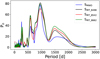 |
Fig. 3 Periodograms of all four time series. |
5.3 Activity cycles
As evidenced by Fig. 2, all Call activity indices increase with time, possibly indicating the presence a long-term activity cycle with a cycle period longer than the time span of the available TIGRE data; a possible long-term cycle will be discussed in Sect. 5.3.2. Furthermore, a shorter and periodic variation on a timescale of years is apparent, which we studied next.
5.3.1 Short-term activity cycle
Before examining these shorter timescale variations, we removed the long-term trend by subtracting a linear relation, to avoid it influencing our period estimation; the estimated linear trends are depicted as dashed lines in each panel of Fig. 2, and in Fig. 4 we plot the detrended time series. Finally, we performed the GLS analysis for the four time detrended series and show the derived GLS periodograms in Fig. 3. Since the SMWO time series has a larger number of data points than the time series of the IRT S-values, we used the corresponding normalised periodograms (Pn) to distinguish the periodograms they are colour-coded for the four different indices. In Fig. 3, a clear peak at nearly the same period appears in all four time series, and we list the values of these four periods and the corresponding formal FAP values in Table 4. The formal FAP values indicate a high significance of the estimated cycle period, and finally, we computed a mean cycle period (see Sect. 5.2) of 949 ± 5 days (≈2.6 yr).
To better visualise the cyclic variations in the individual time series, we fitted the detrended S-index time series with a sine function of the form
 (6)
(6)
where Acyc denotes the amplitude, t time, Pcyc the obtained cycle period (as listed in Table 4), φ the phase at time zero, and b a constant value. Furthermore, we used the mean cycle period of 949 days to perform the sine fit again and these results are similar with the sine fits where the individual cycle periods used and were plotted as a solid black line in Fig. 4. Our choice of a sine function is arbitrary, yet Fig. 4 demonstrates that these sine curves follow the data very well for all four time series.
5.3.2 Evidence of a possible long-term activity cycle
As already mentioned, the SMWO values show a positive trend, which may indicate a possible long-term cycle, yet the time span of the TIGRE data is too short to determine a reliable cycle period. However, in the Isaacson & Fischer (2010) catalogue, five SMWO values are listed, three of which were taken in 2005 and 2006 and two at the end of 2009. Furthermore, in the Wright et al. (2004) catalogue, two SMWO values are listed, which were taken in 1997 and 2001. With these values, we were able to extend our TIGRE SMWO time series, and we show this combined time series in Fig. 5, where the SMWO values are plotted by Wright et al. (2004) in green, values by Isaacson & Fischer (2010) in red and the TIGRE SMWO values in blue; the SMWO values by Wright et al. (2004) and by Isaacson & Fischer (2010) show a decreasing trend while the TIGRE data increase.
To assess the possible cycle period, we studied two different possible cycle lengths. First, we estimated a cycle length based on the maximum value by Wright et al. (2004) at 1997 and the maximum of the TIGRE data at 2021. Based on the data, we assumed that this time range covers two activity cycles with a corresponding cycle length of about 12 yr. The second case was estimated assuming that the maximum value listed by Isaacson & Fischer (2010) and the maximum of the TIGRE data at 2021 correspond to the cycle period, which yields a value of about 15 yr. We performed sine fits, using Eq. (6), with both periods, the results are shown in Fig. 5, with the 12-yr sine fit shown as a dashed red line and the 15-yr sine fit as a dashed black line. The corresponding amplitudes and phases are listed in Table 5. Next, we also performed double sine fits of the form
 (7)
(7)
where the parameters have the same definition as in Eq. (6). Additionally, the label L denotes the parameter for the long-term cycle and S for the 2.6 yr short-term cycle. Again, we performed these fits using both possible long-term estimates and the short cycle period to visualise how well the data are described. We overplot these results in Fig. 5 and list the respective fit values in Table 5. A comparison of the fit amplitudes shows an increase if one considers the possible long- and the short-term cycle for a sine fit. Furthermore, the amplitudes for the possible long- and the short-term cycles are equal inside the error margin. This indicates that the strength of the variation caused by stellar activity are the same for the possible long- and the short-term cycle.
The standard deviation of both fits are similar, so we conclude that the available data are consistent with the presence of a long-term cycle, the period of which is in the range 12–15 yr. A more extended time series is clearly required to better characterise this possible cycle.
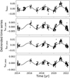 |
Fig. 4 Detrended S-index time series. The solid black line in each panel shows the sine fit with the mean cycle period of 949 days. |
Cycle estimations from the periodogram analysis.
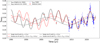 |
Fig. 5 Extended SMWO time series. The green point originates from the Wright et al. (2004) catalogue, the black points are from the Isaacson & Fischer (2010) catalogue, the blue points are TIGRE SMWO values, and the red diamonds represent the observational seasonal mean SMWO values. The dashed lines depict a sine fit with a period of 12 yr (dashed red line) and 15 yr (dashed black line). The solid lines depict double sine fits (the colour-code is the same as for the single sine fits), where the short-term cycle period of 2.6 yr is also considered. |
Parameter long-term cycle estimations.
5.4 Comparison of chromospheric and coronal properties
After determining the 950 days cycle in the chromospheric indicators, we want to find out whether the activity cycle can be detected in X-ray flux as a coronal activity indicator as well. The X-ray telescope SRG (Spectrum-Roentgen-Gamma)/eROSITA (Predehl et al. 2021) scanned HD 111395 during each of the four all-sky surveys it conducted so far. Therefore, we have four X-ray flux measurements, which are taken about 180 days apart. We employed the most recent (preliminary) catalogue data using the processing results from the current version of the eSASS (eROSITA Science Analysis Software System) pipeline, version c020 (Brunner et al. 2022), and extracted the catalogue data from a single X-ray band (0.2-2.3 keV). To convert the measured catalogue count rates to X-ray fluxes, we followed the procedure described in Fuhrmeister et al. (2022), using an energy conversion factor of 0.9 × 10⁻¹² erg cm−2 cnt−1.
Although the eROSITA data are too sparse to detect the activity cycle of HD 111395 in X-rays, a visual comparison between SMWO data and the X-ray fluxes shown in Fig. 6 strongly suggests that the observed long-term variation in the X-ray flux as measured by eROSITA is caused by the activity cycle of HD 111395.
Results of the rotation period determination.
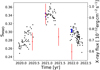 |
Fig. 6 Comparison between SMWO (black dots, left y-axis) and X-ray flux (red dots, right y-axis) measurements. The blue diamonds mark SMWO values from quasi-simultaneous optical observations, which were taken within three days of the X-ray measurement. |
5.5 Rotation period
To determine the rotation period of HD 111395 spectroscopically, we separately investigated the four Call time series obtained in the individual observation seasons; we note that these time series are essentially independent from each other. We applied the same procedure as for the cycle estimation, namely, we first removed a trend in the data and then carried out a GLS analysis. From the periodogram of each season the highest peak and hence the most probable periods are extracted and only the periods with a significance greater than 2σ are listed in Table 6; the corresponding periodograms are shown in Fig. 7; in Appendix A, we plot all seasonal time series with a period significance greater than 2σ to demonstrate our period analysis.
In all seasons, we find a rotation period with a significance of at least 99%, yet the obtained rotation periods with a significance of 3σ vary from 15.12 to 18.92 days. This variation is also visible in the periodograms for the individual observation seasons as seen in Fig. 7. Furthermore, a comparison of the seasonal rotation periods derived from our four indices (see Table 6) shows that the rotation periods in the same season usually agree to within the 2σ error margin.
To obtain a seasonal mean rotation period for the individual seasons, we averaged the listed individual seasonal rotation periods for the different lines. Furthermore, we estimated a FAP value for the seasonal mean rotation period. This averaging of the rotation periods and the estimation of the corresponding FAP is described in Sect. 5.2, and the results are given in Table 6. The comparison of these seasonal values shows a strong scatter of the individual seasonal values. To quantify this scatter, we computed a standard deviation of 1.08 days for these seasonal rotation periods. With a mean rotation period of 16.76 ± 0.36 d as computed from these seasonal mean rotation periods, we then calculated a relative scatter (the ratio between standard deviation and mean rotation period) of ~ 6%.
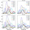 |
Fig. 7 Periodograms of the seasonal GLS analysis where the most probable periods have a significance greater than 2σ. |
5.6 Evidence of stellar differential rotation
Differential rotation in a star manifests itself as change of the stellar rotation period depending on the latitude. The simplest way to describe differential rotation is by introducing a parameter α, defined as the relative change between the equatorial and polar rotation rate through
 (8)
(8)
where Ωpol the rotation rate (2π/Prot) at the stellar pole and Ωeq the rotation rate at equator. Differential rotation is well known for the Sun, where one observes α ≈ 0.3, typically by investigating the relative motions of sunspots, which we do in Sect. 5.6.1.
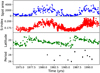 |
Fig. 8 Variations in the Sun. The upper panel shows the variation in the total sunspot area, the second panel the SMWO values from the Mount Wilson programme, the third panel the mean weighted latitude of the sunspots, and the last panel the rotation periods. In the bottom panel, the black dots denote our own rotation period measurements. |
5.6.1 Lessons from the Sun
We next considered the case of the Sun and ask to what extent we would be able to deduce the Sun’s differential rotation from full-disk solar measurements; similar studies have been carried out by Donahue (1993) using S-index data and Donahue & Keil (1995) using solar daily K-line data from the Sacramento Peak Observatory. Here we considered solar S-index data obtained in the context of the Mount Wilson Project, which have been publicly released4 for the time range from 1966.6 to 1992.3 yr. For sunspots, we used the Royal Greenwich Observatory – USAF/NOAA data5, where the total sunspot area (in units of millionths of a hemisphere) is provided as a function of time expressed in a Carrington rotation number for 50 latitude bins uniformly distributed in the sine of solar latitude. In Fig. 8 we plot the total sunspot area derived from these data (upper panel), the Ca II Mount Wilson S-index from 1973 to 1992.3 (second panel from top), the mean weighted latitude of the sunspots (third panel from top) and the rotation period derived by us from the S-index data (bottom panel) from 1973 to 1992.3. As for the bottom panel, a few remarks are in order: solar Mount Wilson S-index data were only sparsely recorded until 1985, and for epochs before 1973 they were recorded very poorly; therefore, we did not use these data. To find a significant rotational signal, we tested different data chunks with individual lengths from 0.5 up to 2 yr, requiring at least one data point every 6 days on average. The Prot was determined in the same fashion as the other periods reported in this paper, except that we used the method by Horne & Baliunas (1986) to determine the Prot because the GLS method requires error values, which are not given for the solar S-index values. The determined Prot values are plotted in the lower panel of Fig. 8 and have a formal significance better than 3σ.
Our so derived solar rotation periods vary from 25.95 ± 0.21 to 29.36 ± 0.18 days.
Figure 8 demonstrates the good correlation between the solar spot area and the S-index. The mean emergence latitude shows a sawtooth behaviour, with a rapid increase over 2 – 3 yr, followed by a decay towards smaller periods (i.e. lower latitudes). Naively, one would expect the rotation period to follow this sawtooth behaviour.
To study the cycle dependence of S-index values, latitude and rotation period, we phase-folded the data and plot them in Fig. 9. For the phase-folding, we used a cycle length of 10.2 yrs, which is the mean of the listed cycle lengths for solar cycles 21 and 22, as provided on the SIDC (Solar Influences Data analysis Center) web page6. As the zero point for the cycle phase, we used the cycle minimum between the solar cycle 21 and 22, which we estimated by performing a sine fit with the mean cycle period of 10.2 yr. This procedure results in a minimum at 1985.9 yr, which is equal to the starting of solar cycle 22 as derived by Egeland et al. (2017), but slightly different than the value from September 1986 (1986.75 yr) provided by the SIDC web page. Figure 9 suggests that the rotation periods follow the sawtooth behaviour of the latitude but the sine-like behaviour of the S-index values.
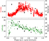 |
Fig. 9 Upper panel: phase-folded S-values (red dots) vs. cycle phase and rotation periods (black circles) vs. cycle phase. Lower panel: phase-folded latitude from 1973 to 1993 (green dots) vs. cycle phase and rotation periods (black circles) vs. cycle phase. |
5.6.2 Variation in the rotation period
We now turn to HD 111395 and plot – in Fig. 7 – the individual periodograms obtained for the estimated rotation periods; obviously one notices strong variations in the most probable periods, but whether or not these variations are actually periodic is hard to see. Therefore, we constructed a 2D time-power diagram, shown in Fig. 10, from the periodograms of the individual seasons, with the x-axis corresponding to the period and the y-axis to time; we note that we ignored periodograms in which the most probable periods were below 2σ. For a better visualisation of the position of the most probable period in these images, these are marked with a vertical solid red line in the 2D images for the four S-index time series are shown in Fig. 10. In these 2D images of the periodogram intensity, a temporal and a periodic variation in all four time series can be noticed.
Furthermore, in Fig. 7, a double-peak structure is visible for all main peaks in the periodograms of the different indices for the seasons of 2018.3 and 2022.1. This double-peak structure suggests the existence of a further rotation period signal produced by an additional plage region. To test the significance of this secondary period, we removed the main period from the seasonal S-index data and found that the secondary signal in the 2018.3 data becomes insignificant but not in the 2022.1 time series. Therefore, in Fig. 11 we show the periodogram of the detrended SMWO time series for the season 2022.1 as black curve. Here, a double-peak structure is apparent, with the main peak at 15.12 ± 0.08 d and a clear deformation in the flank of this peak at ~17.3 days, which indicates a secondary rotational signal. After removing the 15.12 days period from the data, we performed a new GLS analysis of the residuals to obtain a new periodogram, shown in 11 as a red line. Here, a remaining peak at 17.25 ± 0.22 d is apparent, for which we deduced a formal FAP of 0.016 (i.e. close to 3σ). Furthermore, for the bluest of the Ca II IRT lines a similar procedure reveals a persistent peak at 17.27 ± 0.21 d with a FAP of 0.028. The persistence of this additional peak in the periodogram in two independently measured indices can be interpreted as an indication for a second periodic signal in the data.
Next we studied to what extent the measured seasonal mean rotation periods are related to the activity cycle. We first tested whether the measured seasonal mean rotation periods can be considered constant: a χ2-test rejects the null-hypothesis (i.e. rotation periods are constant) with a confidence of 0.99998. Clearly, the computed confidences do depend on the size of the errors, but if we were to increase these errors by an order of magnitude (!), the rotations periods would still have to be considered as non-constant at the 2σ level. We therefore conclude that the measured seasonal mean rotation periods are not constant.
To test whether they show a solar-like behaviour, we phase-folded the seasonal mean rotation periods with the period of the activity cycle length of 949 d, with the zero point set at the first cycle minimum ~2014.7, and applied the same folding procedure to the detrended S-index data. In Fig. 12 we plot the phase-folded S-index data (as shown in the top panel of Fig. 4), the mean seasonal S-index data as well as the derived seasonal rotation periods, to allow for an easy comparison between the S-index values and the length of the rotation period with respect to cycle phase as shown for the Sun in Fig. 9.
Having shown that the derived rotation periods are not constant, an inspection of the distribution of the rotation periods with phase (see Fig. 12) indicates a systematic behaviour, which we can describe, for example, with a ‘triangular’ rotation law, as known from the Sun. To quantify this law, we estimated the trends for both flanks with the boundary condition that at phase 0 and 1 the period equals the minimal rotation period of 15.25 days, and we plot the results as dashed black line in Fig. 12. We computed a standard deviation of 0.6 days for the residuals, which represents a clear reduction in the scatter compered to 1.07 days, assuming a constant rotation period. To test the significance of this reduction, we performed an F-test and obtained a p-value of 0.00075, which implies that the triangular shape describes the rotation periods versus phase better with a significance of 99.93% as compared to the assumption of a constancy of the rotation periods.
Clearly, other analytical shapes of the assumed rotation law would also yield good descriptions, the shape chosen above is not unique, but we do conclude that the variation in the rotation period is significant and systematic, and may even show some resemblance to the sawtooth behaviour known from the Sun. However, we caution that the phase coverage of the rotation periods should be improved to better understand the variations in the measured periods. Therefore, spectroscopically covering a few more activity cycles of HD 111395 would be highly desirable.
Finally, we estimated the differential rotation parameter, a, from observed minimum and maximum values of the measured rotation rates through
 (9)
(9)
We find a value of αmax−min = 0.1922 ± 0.0040 for the case of HD 111395. From our minimal and maximal determined solar rotation periods given in Sect. 5.6.1, we also computed with Eq. (9) an α-value and obtained αmax−min = 0.1161 ± 0.0090. The comparison of both αmax−min values shows a lower value for the differential rotation shear of the Sun and this indicates a stronger differential rotation in HD 111395 than in our Sun.
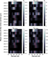 |
Fig. 10 Intensity plot of the individual periodograms (Pn) of the different observation seasons. The y-axis shows the mean time of each season, and the x-axis the period. The positions of the most probable periods –listed in Table 6 – are marked with a vertical solid red line. |
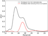 |
Fig. 11 Periodogram of the detrended SMWO time series with the seasonal mean of 2022.1 (black curve; compare with Fig. 7). The red curve shows the periodogram of the same time series but with the 15.12 days period removed. |
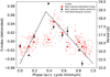 |
Fig. 12 Detrended S-index vs. cycle phase (red dots). For comparison, we overplot the seasonal mean rotation period (black circles) and the seasonal mean S-indices (red circles). The dashed black line shows the estimated trends for both flanks to visualise the assumed ‘triangular’ rotation law. |
6 Cycle and activity of HD 111395 in a global context
In this section we present our results of HD 111395 in a more global context. For this, we compared the determined cycle and mean rotation period of HD 111395 with the general cycle–rotation relation. We also compared the chromospheric and coronal activity level of HD 111395 with the other stars that show an activity cycle in X-rays.
6.1 Cycle–rotation connection
As mentioned before, the total number of stars with a well-known activity cycle is quite low. In the recent paper by Mittag et al. (2023) a list of 44 main-sequence stars with well-determined cycles is presented, and we used these stars to check how the 2.6 yr short-term cycle and a possible long-term cycle with a cycle length in the time range of 12–15 yr fit into the cycle–rotation relation.
In Fig. 13, we plot the logarithm of the cycle period versus the logarithm of the rotation period; the stars with two cycles known are marked and connected with a dashed blue line. Clearly, both the 2.6 yr short-term cycle of HD 111395 (marked as a blue star) and the long-term cycle (12 and 15 yr; marked as magenta and yellow stars) fits very well into the known cycle–rotation relations.
The same applies when one uses the Rossby number as activity indicator: Mittag et al. (2023) show that there colour-dependent branches in a cycle length versus Rossby number representation. In Fig. 14 we plot the logarithm of the short-term cycles from Mittag et al. (2023) including the 2.6 yr cycle of HD 111395 versus the logarithm of the corresponding Rossby numbers, where the different B – V range colour-coded.
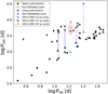 |
Fig. 13 Logarithm of the cycle period versus the logarithm of the rotation period. The dots indicate the cycle on the short-cycle branch, and diamonds the cycle on the long-cycle branch. The stars show the position of HD 111395 in the cycle-rotation presentation. The cycles for the same object are connected with a dashed line. |
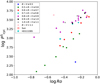 |
Fig. 14 Logarithm of the cycle period located on the short-cycle branch versus the logarithm of Rossby number. The dataset is split into different B – V ranges and colour-coded. The star symbol marks the position of HD 111395 in the cycle-Rossby number representation. |
6.2 Chromospheric and coronal activity levels of HD 111395
Here, we briefly discuss and compare the chromospheric and coronal activity levels of HD 111395 with other late-type stars with known cycles. Using the activity index  , which is the pure Ca II flux excess (Mittag et al. 2013), we plot (in Fig. 15 versus the colour index B – V for the sample stars presented by Mittag et al. 2023). Clearly, HD 111395 belongs to the more active stars, and using the log
  value of −5.05 for our Sun listed in Mittag et al. (2023) we conclude that HD 111395 is more chromospherically active than the Sun by a factor of 3.7, yet its chromospheric activity level is comparable to those of other cyclic stars.
Turning now to coronal emission, we first note that the detection of activity cycles in X-rays is quite difficult because of very limited observation possibilities in terms of data sampling. Thus, there are only a few stars with known X-ray activity cycles and the vast majority of activity cycles were discovered via ‘traditional’ S-index measurements with the exception of HD 128620 and HD 128621 (= α Cen A and B). Our comparison of the S-index and X-ray time series of HD 111395 as shown in Fig. 12 suggests that the activity cycle of HD 111395 is also visible in its X-ray flux, but clearly more observations are required to confirm this finding. For comparison, we list those stars with a coronal activity cycle measured through X-ray emission including HD 111395 in Table 7, which shows that X-ray cycles are found in stars considerably more active than the Sun. Furthermore, Table 7 reveals that the detected X-ray cycle periods are typically below 10 yrs, except for the Sun and HD 128620. This is clearly an observational bias. To find long-term cycles one needs time series longer than 10 yrs with high precision to see cyclic variations, which is quite difficult especially in the X-ray range.
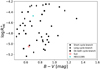 |
Fig. 15 Logarithm of the activity index |

7 Discussion and conclusions
In this paper, we present the results of our stellar activity study of the bright star HD 111395 with respect to its photospheric, chromospheric, and coronal activity properties. All these data indicate that HD 111395 is far more active than the Sun and other stars with well-known activity cycles. Our time series of Ca II H&K and IRT data obtained from nine years of TIGRE observations of HD 111395 shows both long-term and short-term variations. The long-term variations in the Ca II H&K and IRT data are caused by activity cycles; we determined an activity cycle length of 949 d (≈2.6 yr); there is also some evidence for a possible longer-term cycle with periods of the order of 12–15 yr. The TIGRE Ca II H&K and IRT time series also show short-term variations in each season, which we attribute to stellar rotation with a mean rotation period of 16.76 ± 0.36 d for HD 111395.
The derived seasonal mean rotation periods show a highly significant and systematic variation in the range 15.25–18.88 days. The observed variations appear to be related to the phase in the activity cycle and are therefore interpreted as signatures of stellar differential rotation. HD 111395 shows a phenomenological behaviour very much reminiscent of the Sun despite its much higher activity level. Finally, we estimated the differential rotation parameter, α, and find an αmax−min of 0.1922, a value larger than the corresponding solar value.
In a more general context, we investigated how our findings relate to the cycle–rotation relation and find that both the short-term cycle and the possible longer-term cycle fit very well into the known cycle–rotation relation. Needless to say, more observations are required to determine the length of this possible long-term cycle, while we consider the period of the short-term cycle to be well established.
Our results demonstrate that HD 111395 is a very interesting test case for the study of stellar activity. The nature of the longer-term cycle remains unclear, and a larger number of rotation measurements over a longer period of time would be highly desirable. As the stability of the cycle periods deserves further study, we are continuing our monitoring of HD 111395 with TIGRE.
Stars with X-ray cycles.
Acknowledgements.
This work is based on data from eROSITA, the soft X-ray instrument aboard SRG, a joint Russian-German science mission supported by the Russian Space Agency (Roskosmos), in the interests of the Russian Academy of Sciences represented by its Space Research Institute (IKI), and the Deutsches Zentrum für Luft- und Raumfahrt (DLR). The SRG spacecraft was built by Lavochkin Association (NPOL) and its subcontractors, and is operated by NPOL with support from the Max Planck Institute for Extraterrestrial Physics (MPE). The HK_Project_v1995_NSO data derive from the Mount Wilson Observatory HK Project, which was supported by both public and private funds through the Carnegie Observatories, the Mount Wilson Institute, and the Harvard-Smithsonian Center for Astrophysics starting in 1966 and continuing for over 36 yr. These data are the result of the dedicated work of O. Wilson, A. Vaughan, G. Preston, D. Duncan, S. Baliunas, and many others. This paper includes data collected with the TESS mission, obtained from the MAST data archive at the Space Telescope Science Institute (STScI). Funding for the TESS mission is provided by the NASA Explorer Program. STScI is operated by the Association of Universities for Research in Astronomy, Inc., under NASA contract NAS 5-26555. This research has made valuable use of the VizieR catalogue access tool, CDS, Strasbourg, France. The original description of the VizieR service was published in Ochsenbein et al. (2000). J.R. acknowledges support from the DLR under grant 50QR2105.
Appendix A Seasonal time series
Here, we show plots to illustrate our analysis of the seasonal time series carried out to determine the rotation periods, which are listed in Table 6. The upper panel shows the seasonal time series. For cases where we do not find a trend, we show the sine curve with the period that we found as a red line. If we found a trend, this trend is plotted in the graphs; in the middle panel, we show the time series where this trend is removed and show the sine curve with the period that we found as a red line. In the lower two panels, we show on the left-hand side the periodogram obtained from the GLS analysis (upper part) and the window function (lower part), and on the right-hand side we show the phased-folded time series, with the phased-folded sine fit as a solid red line.
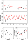 |
Fig. A.1 SMWO time series analysis from season 2014.2. |
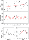 |
Fig. A.2 SMWO time series analysis from season 2015.2. |
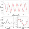 |
Fig. A.3 SMWO time series analysis from season 2016.2. |
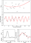 |
Fig. A.4 SMWO time series analysis from season 2017.3. |
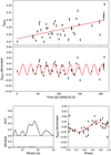 |
Fig. A.5 SMWO time series analysis from season 2018.3. |
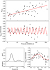 |
Fig. A.6 SMWO time series analysis from season 2020.2. |
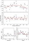 |
Fig. A.7 SMWO time series analysis from season 2021.1. |
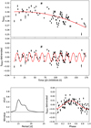 |
Fig. A.8 SMWO time series analysis from season 2022.1. |
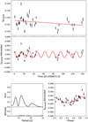 |
Fig. A.9 SIRT8498 time series analysis from season 2014.2. |
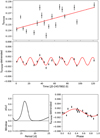 |
Fig. A.10 SIRT8498 time series analysis from season 2017.3. |
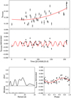 |
Fig. A.11 SIRT8498 time series analysis from season 2018.3. |
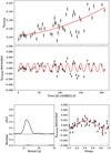 |
Fig. A.12 SIRT8498 time series analysis from season 2020.2. |
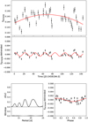 |
Fig. A.13 SIRT8498 time series analysis from season 2021.1. |
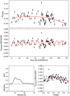 |
Fig. A.14 SIRT8498 time series analysis from season 2022.1. |
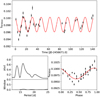 |
Fig. A.15 SIRT8542 time series analysis from season 2014.2. |
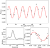 |
Fig. A.16 SIRT8542 time series analysis from season 2016.2. |
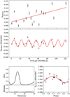 |
Fig. A.17 SIRT8542 time series analysis from season 2017.3. |
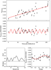 |
Fig. A.18 SIRT8542 time series analysis from season 2018.3. |
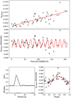 |
Fig. A.19 SIRT8542 time series analysis from season 2020.2. |
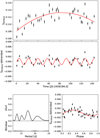 |
Fig. A.20 SIRT8542 time series analysis from season 2021.1. |
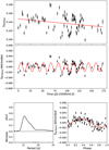 |
Fig. A.21 SIRT8542 time series analysis from season 2022.1. |
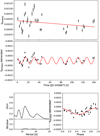 |
Fig. A.22 SIRT8662 time series analysis from season 2014.2. |
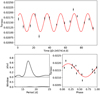 |
Fig. A.23 SIRT8662 time series analysis from season 2016.2. |
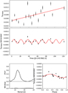 |
Fig. A.24 SIRT8662 time series analysis from season 2017.3. |
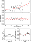 |
Fig. A.25 SIRT8662 time series analysis from season 2018.3. |
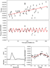 |
Fig. A.26 SIRT8662 time series analysis from season 2020.2. |
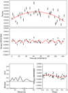 |
Fig. A.27 SIRT8662 time series analysis from season 2021.1. |
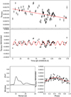 |
Fig. A.28 SIRT8662 time series analysis from season 2022.1. |
References
- Ayres, T. R. 2020, ApJS, 250, 16 [NASA ADS] [CrossRef] [Google Scholar]
- Baliunas, S. L., Donahue, R. A., Soon, W. H., et al. 1995, ApJ, 438, 269 [Google Scholar]
- Basri, G., & Shah, R. 2020, ApJ, 901, 14 [Google Scholar]
- Baum, A. C., Wright, J. T., Luhn, J. K., & Isaacson, H. 2022, AJ, 163, 183 [NASA ADS] [CrossRef] [Google Scholar]
- Böhm-Vitense, E. 2007, ApJ, 657, 486 [CrossRef] [Google Scholar]
- Boro Saikia, S., Marvin, C. J., Jeffers, S. V., et al. 2018, A&A, 616, A108 [NASA ADS] [CrossRef] [EDP Sciences] [Google Scholar]
- Brandenburg, A., Mathur, S., & Metcalfe, T. S. 2017, ApJ, 845, 79 [NASA ADS] [CrossRef] [Google Scholar]
- Brunner, H., Liu, T., Lamer, G., et al. 2022, A&A, 661, A1 [NASA ADS] [CrossRef] [EDP Sciences] [Google Scholar]
- Cayrel de Strobel, G. 1996, A&ARv, 7, 243 [CrossRef] [Google Scholar]
- Coffaro, M., Stelzer, B., Orlando, S., et al. 2020, A&A, 636, A49 [EDP Sciences] [Google Scholar]
- Donahue, R. A. 1993, PhD Thesis, New Mexico State University, USA [Google Scholar]
- Donahue, R. A., & Keil, S. L. 1995, Sol. Phys., 159, 53 [NASA ADS] [CrossRef] [Google Scholar]
- Donahue, R. A., Saar, S. H., & Baliunas, S. L. 1996, ApJ, 466, 384 [Google Scholar]
- Eberhard, G., & Schwarzschild, K. 1913, ApJ, 38 [Google Scholar]
- Egeland, R., Soon, W., Baliunas, S., et al. 2017, ApJ, 835, 25 [NASA ADS] [CrossRef] [Google Scholar]
- ESA 1997, The Hipparcos and Tycho Catalogues, ESA SP-1200 [Google Scholar]
- Fuhrmeister, B., Czesla, S., Robrade, J., et al. 2022, A&A, 661, A24 [NASA ADS] [CrossRef] [EDP Sciences] [Google Scholar]
- Gaia Collaboration 2018, VizieR Online Data Catalog: I/345 [Google Scholar]
- Gaia Collaboration 2022, VizieR Online Data Catalog: I/355 [Google Scholar]
- Głębocki, R. & Gnaciński, P. 2005, ESA Spec. Pub., 560, 571 [Google Scholar]
- González-Pérez, J. N., Mittag, M., Schmitt, J. H. M. M., et al. 2022, Front. Astron. Space Sci., 9, 912546 [CrossRef] [Google Scholar]
- Gray, D. F. 2005, The Observation and Analysis of Stellar Photospheres (Cambridge University Press) [Google Scholar]
- Gray, R. O., Corbally, C. J., Garrison, R. F., McFadden, M. T., & Robinson, P. E. 2003, AJ, 126, 2048 [Google Scholar]
- Hall, J. C., Lockwood, G. W., & Skiff, B. A. 2007, AJ, 133, 862 [Google Scholar]
- Hempelmann, A., Mittag, M., Gonzalez-Perez, J. N., et al. 2016, A&A, 586, A14 [NASA ADS] [CrossRef] [EDP Sciences] [Google Scholar]
- Horne, J. H., & Baliunas, S. L. 1986, ApJ, 302, 757 [Google Scholar]
- Hünsch, M., Schmitt, J. H. M. M., Sterzik, M. F., & Voges, W. 1999, A&AS, 135, 319 [CrossRef] [EDP Sciences] [Google Scholar]
- Isaacson, H. & Fischer, D. 2010, ApJ, 725, 875 [NASA ADS] [CrossRef] [Google Scholar]
- Kopp, G., & Lean, J. L. 2011, Geophys. Res. Lett., 38, L01706 [Google Scholar]
- Martin, J., Fuhrmeister, B., Mittag, M., et al. 2017, A&A, 605, A113 [NASA ADS] [CrossRef] [EDP Sciences] [Google Scholar]
- Metcalfe, T. S., & van Saders, J. 2017, Sol. Phys., 292, 126 [NASA ADS] [CrossRef] [Google Scholar]
- Metcalfe, T. S., Basu, S., Henry, T. J., et al. 2010, ApJ, 723, L213 [NASA ADS] [CrossRef] [Google Scholar]
- Metcalfe, T. S., Buccino, A. P., Brown, B. P., et al. 2013, ApJ, 763, L26 [Google Scholar]
- Metcalfe, T. S., Egeland, R., & van Saders, J. 2016, ApJ, 826, L2 [Google Scholar]
- Metcalfe, T. S., Finley, A. J., Kochukhov, O., et al. 2022, ApJ, 933, L17 [NASA ADS] [CrossRef] [Google Scholar]
- Mittag, M., Hempelmann, A., González-Perez, J. N., & Schmitt, J. H. M. M. 2010, Adv. Astron., 2010, 101502 [CrossRef] [Google Scholar]
- Mittag, M., Schmitt, J. H. M. M., & Schröder, K.-P. 2013, A&A, 549, A117 [NASA ADS] [CrossRef] [EDP Sciences] [Google Scholar]
- Mittag, M., Schröder, K. P., Hempelmann, A., González-Pérez, J. N., & Schmitt, J. H. M. M. 2016, A&A, 591, A89 [NASA ADS] [CrossRef] [EDP Sciences] [Google Scholar]
- Mittag, M., Hempelmann, A., Schmitt, J. H. M. M., et al. 2017a, A&A, 607, A87 [NASA ADS] [CrossRef] [EDP Sciences] [Google Scholar]
- Mittag, M., Robrade, J., Schmitt, J. H. M. M., et al. 2017b, A&A, 600, A119 [NASA ADS] [CrossRef] [EDP Sciences] [Google Scholar]
- Mittag, M., Schmitt, J. H. M. M., Hempelmann, A., & Schröder, K. P. 2019, A&A, 621, A136 [NASA ADS] [CrossRef] [EDP Sciences] [Google Scholar]
- Mittag, M., Schmitt, J. H. M. M., & Schröder, K. P. 2023, A&A, 674, A116 [NASA ADS] [CrossRef] [EDP Sciences] [Google Scholar]
- Newton, H.W., & Nunn, L. 1951, MNRAS, 111, 413 [NASA ADS] [CrossRef] [Google Scholar]
- Noyes, R. W., Weiss, N. O., & Vaughan, A. H. 1984, ApJ, 287, 769 [Google Scholar]
- Olspert, N., Lehtinen, J. J., Käpylä, M. J., Pelt, J., & Grigorievskiy, A. 2018, A&A, 619, A6 [NASA ADS] [CrossRef] [EDP Sciences] [Google Scholar]
- Ochsenbein, F., Bauer, P., & Marcout, J. 2000, A&AS, 143, 23 [NASA ADS] [CrossRef] [EDP Sciences] [Google Scholar]
- Parker, E. N. 1955, ApJ, 122, 293 [Google Scholar]
- Pojmanski, G. 1997, Acta Astron., 47, 467 [Google Scholar]
- Predehl, P., Andritschke, R., Arefiev, V., et al. 2021, A&A, 647, A1 [EDP Sciences] [Google Scholar]
- Radick, R. R., Lockwood, G. W., Henry, G. W., Hall, J. C., & Pevtsov, A. A. 2018, ApJ, 855, 75 [Google Scholar]
- Reinhold, T., Reiners, A., & Basri, G. 2013, A&A, 560, A4 [NASA ADS] [CrossRef] [EDP Sciences] [Google Scholar]
- Ricker, G. R., Winn, J. N., Vanderspek, R., et al. 2015, J. Astron. Telesc. Instrum. Sys., 1 014003. [Google Scholar]
- Robrade, J., Schmitt, J. H. M. M., & Favata, F. 2012, A&A, 543, A84 [NASA ADS] [CrossRef] [EDP Sciences] [Google Scholar]
- Saar, S. H., & Baliunas, S. L. 1992, ASP Conf. Ser., 27, 150 [NASA ADS] [Google Scholar]
- Sanz-Forcada, J., Stelzer, B., & Metcalfe, T. S. 2013, A&A, 553, L6 [NASA ADS] [CrossRef] [EDP Sciences] [Google Scholar]
- Schmitt, J. H.M.M., & Mittag, M. 2020, Astron. Nachr., 341, 497 [NASA ADS] [CrossRef] [Google Scholar]
- Schmitt, J. H. M. M., Schröder, K.-P., Rauw, G., et al. 2014, Astron. Nachr., 335, 787 [NASA ADS] [CrossRef] [Google Scholar]
- Schröder, K. P., Mittag, M., Jack, D., Rodríguez Jiménez, A., & Schmitt, J. H. M. M. 2020, MNRAS, 492, 1110 [CrossRef] [Google Scholar]
- Schwabe, H. 1844, Astron. Nachr., 21, 233 [Google Scholar]
- Smith, J. C., Stumpe, M. C., Van Cleve, J. E., et al. 2012, PASP, 124, 1000 [Google Scholar]
- Soubiran, C., Le Campion, J.-F., Brouillet, N., & Chemin, L. 2016, A&A, 591, A118 [NASA ADS] [CrossRef] [EDP Sciences] [Google Scholar]
- Strassmeier, K. G., Serkowitsch, E., & Granzer, T. 1999, A&AS, 140, 29 [NASA ADS] [CrossRef] [EDP Sciences] [Google Scholar]
- Stumpe, M. C., Smith, J. C., Van Cleve, J. E., et al. 2012, PASP, 124, 985 [Google Scholar]
- Suárez Mascareño, A., Rebolo, R., & González Hernández, J. I. 2016, A&A, 595, A12 [Google Scholar]
- Tuominen, I., Rüdiger, G., & Brandenburg, A. 1988, in Activity in Cool Star Envelopes, eds. O. Havnes, B. R. Pettersen, J. H. M. M. Schmitt, & J. E. Solheim, 143, 13 [NASA ADS] [CrossRef] [Google Scholar]
- Vaughan, A. H., Preston, G. W., & Wilson, O. C. 1978, PASP, 90, 267 [Google Scholar]
- Wargelin, B. J., Saar, S. H., Pojmanski, G., Drake, J. J., & Kashyap, V. L. 2017, MNRAS, 464, 3281 [NASA ADS] [CrossRef] [Google Scholar]
- Wilson, O. C. 1978, ApJ, 226, 379 [Google Scholar]
- Wright, J. T., Marcy, G. W., Butler, R. P., & Vogt, S. S. 2004, VizieR Online Data Catalog: J/ApJS/152/261 [Google Scholar]
- Zechmeister, M., & Kürster, M. 2009, A&A, 496, 577 [CrossRef] [EDP Sciences] [Google Scholar]
For a detailed description and to download the data, see https://dataverse.harvard.edu/dataverse/mwo_hk_project
The data compiled by D. Hathaway are available at https://solarscience.msfc.nasa.gov/greenwch.shtml
All Tables
All Figures
|
Fig. 1 Normalised TESS light curves. The left panel shows the light curve taken in 2020 from March 20 to April 15, and the right panel shows the light curve taken in 2022 from February 26 to March 25. |
| In the text | |
|
Fig. 2 Time series of the Ca II activity indices. From top to bottom, the SMWO, SIRT_8498, SIRT_8542, and SIRT_8662 time series are plotted (black dots). The dashed red line in each panel represents the best-fit linear trend. |
| In the text | |
|
Fig. 3 Periodograms of all four time series. |
| In the text | |
|
Fig. 4 Detrended S-index time series. The solid black line in each panel shows the sine fit with the mean cycle period of 949 days. |
| In the text | |
|
Fig. 5 Extended SMWO time series. The green point originates from the Wright et al. (2004) catalogue, the black points are from the Isaacson & Fischer (2010) catalogue, the blue points are TIGRE SMWO values, and the red diamonds represent the observational seasonal mean SMWO values. The dashed lines depict a sine fit with a period of 12 yr (dashed red line) and 15 yr (dashed black line). The solid lines depict double sine fits (the colour-code is the same as for the single sine fits), where the short-term cycle period of 2.6 yr is also considered. |
| In the text | |
|
Fig. 6 Comparison between SMWO (black dots, left y-axis) and X-ray flux (red dots, right y-axis) measurements. The blue diamonds mark SMWO values from quasi-simultaneous optical observations, which were taken within three days of the X-ray measurement. |
| In the text | |
|
Fig. 7 Periodograms of the seasonal GLS analysis where the most probable periods have a significance greater than 2σ. |
| In the text | |
|
Fig. 8 Variations in the Sun. The upper panel shows the variation in the total sunspot area, the second panel the SMWO values from the Mount Wilson programme, the third panel the mean weighted latitude of the sunspots, and the last panel the rotation periods. In the bottom panel, the black dots denote our own rotation period measurements. |
| In the text | |
|
Fig. 9 Upper panel: phase-folded S-values (red dots) vs. cycle phase and rotation periods (black circles) vs. cycle phase. Lower panel: phase-folded latitude from 1973 to 1993 (green dots) vs. cycle phase and rotation periods (black circles) vs. cycle phase. |
| In the text | |
|
Fig. 10 Intensity plot of the individual periodograms (Pn) of the different observation seasons. The y-axis shows the mean time of each season, and the x-axis the period. The positions of the most probable periods –listed in Table 6 – are marked with a vertical solid red line. |
| In the text | |
|
Fig. 11 Periodogram of the detrended SMWO time series with the seasonal mean of 2022.1 (black curve; compare with Fig. 7). The red curve shows the periodogram of the same time series but with the 15.12 days period removed. |
| In the text | |
|
Fig. 12 Detrended S-index vs. cycle phase (red dots). For comparison, we overplot the seasonal mean rotation period (black circles) and the seasonal mean S-indices (red circles). The dashed black line shows the estimated trends for both flanks to visualise the assumed ‘triangular’ rotation law. |
| In the text | |
|
Fig. 13 Logarithm of the cycle period versus the logarithm of the rotation period. The dots indicate the cycle on the short-cycle branch, and diamonds the cycle on the long-cycle branch. The stars show the position of HD 111395 in the cycle-rotation presentation. The cycles for the same object are connected with a dashed line. |
| In the text | |
|
Fig. 14 Logarithm of the cycle period located on the short-cycle branch versus the logarithm of Rossby number. The dataset is split into different B – V ranges and colour-coded. The star symbol marks the position of HD 111395 in the cycle-Rossby number representation. |
| In the text | |
|
Fig. 15 Logarithm of the activity index |
| In the text | |
|
Fig. A.1 SMWO time series analysis from season 2014.2. |
| In the text | |
|
Fig. A.2 SMWO time series analysis from season 2015.2. |
| In the text | |
|
Fig. A.3 SMWO time series analysis from season 2016.2. |
| In the text | |
|
Fig. A.4 SMWO time series analysis from season 2017.3. |
| In the text | |
|
Fig. A.5 SMWO time series analysis from season 2018.3. |
| In the text | |
|
Fig. A.6 SMWO time series analysis from season 2020.2. |
| In the text | |
|
Fig. A.7 SMWO time series analysis from season 2021.1. |
| In the text | |
|
Fig. A.8 SMWO time series analysis from season 2022.1. |
| In the text | |
|
Fig. A.9 SIRT8498 time series analysis from season 2014.2. |
| In the text | |
|
Fig. A.10 SIRT8498 time series analysis from season 2017.3. |
| In the text | |
|
Fig. A.11 SIRT8498 time series analysis from season 2018.3. |
| In the text | |
|
Fig. A.12 SIRT8498 time series analysis from season 2020.2. |
| In the text | |
|
Fig. A.13 SIRT8498 time series analysis from season 2021.1. |
| In the text | |
|
Fig. A.14 SIRT8498 time series analysis from season 2022.1. |
| In the text | |
|
Fig. A.15 SIRT8542 time series analysis from season 2014.2. |
| In the text | |
|
Fig. A.16 SIRT8542 time series analysis from season 2016.2. |
| In the text | |
|
Fig. A.17 SIRT8542 time series analysis from season 2017.3. |
| In the text | |
|
Fig. A.18 SIRT8542 time series analysis from season 2018.3. |
| In the text | |
|
Fig. A.19 SIRT8542 time series analysis from season 2020.2. |
| In the text | |
|
Fig. A.20 SIRT8542 time series analysis from season 2021.1. |
| In the text | |
|
Fig. A.21 SIRT8542 time series analysis from season 2022.1. |
| In the text | |
|
Fig. A.22 SIRT8662 time series analysis from season 2014.2. |
| In the text | |
|
Fig. A.23 SIRT8662 time series analysis from season 2016.2. |
| In the text | |
|
Fig. A.24 SIRT8662 time series analysis from season 2017.3. |
| In the text | |
|
Fig. A.25 SIRT8662 time series analysis from season 2018.3. |
| In the text | |
|
Fig. A.26 SIRT8662 time series analysis from season 2020.2. |
| In the text | |
|
Fig. A.27 SIRT8662 time series analysis from season 2021.1. |
| In the text | |
|
Fig. A.28 SIRT8662 time series analysis from season 2022.1. |
| In the text | |
Current usage metrics show cumulative count of Article Views (full-text article views including HTML views, PDF and ePub downloads, according to the available data) and Abstracts Views on Vision4Press platform.
Data correspond to usage on the plateform after 2015. The current usage metrics is available 48-96 hours after online publication and is updated daily on week days.
Initial download of the metrics may take a while.