| Issue |
A&A
Volume 669, January 2023
|
|
|---|---|---|
| Article Number | A159 | |
| Number of page(s) | 27 | |
| Section | Astrophysical processes | |
| DOI | https://doi.org/10.1051/0004-6361/202244311 | |
| Published online | 26 January 2023 | |
Numerical simulations of MHD jets from Keplerian accretion disks
I. Recollimation shocks
1
Univ. Grenoble Alpes, CNRS, IPAG, 414 rue de la Piscine, 38400 Saint-Martin d’Hères, France
e-mail: thomas.jannaud@univ-grenoble-alpes.fr
2
INAF – Osservatorio Astrofisico di Torino, Strada Osservatorio 20, Pino Torinese 10025, Italy
Received:
20
June
2022
Accepted:
23
October
2022
Context. The most successful scenario for the origin of astrophysical jets requires a large-scale magnetic field anchored in a rotating object (black hole or star) and/or its surrounding accretion disk. Platform jet simulations, where the mass load onto the magnetic field is not computed by solving the vertical equilibrium of the disk but is imposed as a boundary condition, are very useful for probing the jet acceleration and collimation mechanisms. The drawback of such simulations is the very large parameter space: despite many previous attempts, it is very difficult to determine the generic results that can be derived from them.
Aims. We wish to establish a firm link between jet simulations and analytical studies of magnetically driven steady-state jets from Keplerian accretion disks. In particular, the latter have predicted the existence of recollimation shocks – due to the dominant hoop stress –, which have so far never been observed in platform simulations.
Methods. We performed a set of axisymmetric magnetohydrodynamics (MHD) simulations of nonrelativistic jets using the PLUTO code. The simulations are designed to reproduce the boundary conditions generally expected in analytical studies. We vary two parameters: the magnetic flux radial exponent α and the jet mass load κ. In order to reach the huge unprecedented spatial scales implied by the analytical solutions, we used a new method allowing us to boost the temporal evolution.
Results. We confirm the existence of standing recollimation shocks at large distances. As in self-similar studies, their altitude evolves with the mass load κ. The shocks are weak and correspond to oblique shocks in a moderately high, fast magnetosonic flow. The jet emitted from the disk is focused toward the inner axial spine, which is the outflow connected to the central object. The presence of this spine is shown to have a strong influence on jet asymptotics. We also argue that steady-state solutions with α ≥ 1 are numerically out of range.
Conclusions. Internal recollimation shocks may produce observable features such as standing knots of enhanced emission and a decrease in the flow rotation rate. However, more realistic simulations (e.g. fully three-dimensional) must be carried out in order to investigate nonaxisymmetric instabilities and with ejection only from a finite zone in the disk, so as to to verify whether these MHD recollimation shocks and their properties are maintained.
Key words: magnetohydrodynamics (MHD) / methods: numerical / ISM: jets and outflows / galaxies: active
© The Authors 2023
 Open Access article, published by EDP Sciences, under the terms of the Creative Commons Attribution License (https://creativecommons.org/licenses/by/4.0), which permits unrestricted use, distribution, and reproduction in any medium, provided the original work is properly cited.
This article is published in open access under the Subscribe-to-Open model. Subscribe to A&A to support open access publication.
1. Introduction
Astrophysical jets are commonly observed in most, if not all, types of accreting sources. They are emitted from young stellar objects (YSOs; Bally et al. 2007; Ray et al. 2007; Ray & Ferreira 2021), active galactic nuclei (AGNs) and quasars (Boccardi et al. 2017), close interacting binary systems (Fender & Gallo 2014; Tudor et al. 2017), and even post-AGB stars (Bollen et al. 2017). Despite the different central objects (be it a black hole, a protostar, a white dwarf, or a neutron star), these jets share several properties: (i) they are supersonic collimated outflows with small opening angles, (ii) the asymptotic speeds scale with the escape speed from the potential well of the central object, and (iii) they carry away a sizeable fraction of the power released in the accretion disk. As the only common feature shared by all these different astrophysical objects is the existence of an accretion disk, it is natural to seek a jet model that is related to the disk and not to the central engine. This universal approach is further consistent with the accretion–ejection correlations observed in these objects (see e.g., Merloni & Fabian 2003; Corbel et al. 2003; Gallo et al. 2004; Coriat et al. 2011; Ferreira et al. 2006; Cabrit 2007 and references therein).
Despite these general common trends, astrophysical jets do show some differences in their collimation properties. For instance, the core-brightened extragalactic jets, classified as FRI jets after Fanaroff & Riley (1974), appear conical and show large-scale wiggles (see e.g., Laing & Bridle 2013, 2014 and references therein). On the contrary, the edge-brightened FRII jets appear nearly cylindrical, with a terminal hotspot (Laing et al. 1994; Boccardi et al. 2017). Most of the jets imaged with very long baseline interferometry do not appear as continuous flows, but can be modeled as a sum of discrete features, known as blobs or knots, usually associated with shocks (Zensus 1997). Those shocks are assumed to originate either from pressure mismatches at the jet boundary with the external medium or from major changes at the base of the flow (e.g., new plasma ejections or directional changes), with some of these knots being stationary features (e.g., Lister et al. 2009, 2013; Walker et al. 2018; Doi et al. 2018; Park et al. 2019).
On the other hand, jets from young forming stars do not seem to have such a clear FRI/FRII dichotomy and often display evidence of a conflictual interaction (shocks) with the ambient cloud medium (Reipurth & Bally 2001). This might be consistent with the suspicion that the FR dichotomy would only be a consequence of the jet interaction with its environment, with low-power jets remaining undisrupted and forming hotspots in lower mass hosts (Mingo et al. 2019). However, protostellar jets might also have intrinsic collimation properties different from those of extragalactic jets, possibly because they are nonrelativistic outflows. This is an open question.
Since the seminal model of Blandford & Payne (1982; hereafter BP82), it is known that a large-scale vertical magnetic field threading an accretion disk is capable of accelerating the loaded disk material up to super-fast magnetosonic speeds. This acceleration, usually termed magneto-centrifugal, goes along with an asymptotic collimation of the ejected plasma thanks to the magnetic tension associated with the toroidal magnetic field (hoop stress). In this semi-analytical model, a self-similar ansatz has been used allowing the full set of stationary ideal magnetohydrodynamic (MHD) equations to be solved. Later, this self-similar jet model was generalized in different ways by altering the magnetic field distribution (Contopoulos & Lovelace 1994; Ostriker 1997), thermal effects (Vlahakis et al. 2000; Ceccobello et al. 2018) and was even extended to the relativistic regime (Li et al. 1992; Vlahakis & Königl 2003; Polko et al. 2010, 2014). However, it is unclear whether or not self-similarity affects the overall jet collimation properties. Not only are both the axis and the jet-ambient medium region not taken into account, but the final outcome of the jets (i.e., acceleration efficiency, jet kinematics and opening angle, presence of radial oscillations, or even shocks) may well also be impacted by the imposed geometry.
Using the only class of self-similar jet models smoothly connected to a quasi-Keplerian accretion disk, Ferreira (1997; hereafter F97) showed that these super-fast magnetosonic jets systematically undergo a refocusing toward the axis (see also Polko et al. 2010). Such a recollimation is due to the dominant effect of the internal hoop stress and has nothing to do with a pressure mismatch at the jet–ambient medium interface proposed to explain knotty features in extragalactic jets (Komissarov & Falle 1998; Perucho & Martí 2007; Perucho 2020). According to F97, recollimation would be generic to MHD jets anchored over a large range of Keplerian accretion disks. This is indeed verified for warm outflows (Casse & Ferreira 2000a) and weak magnetic fields (Jacquemin-Ide et al. 2019).
While MHD recollimation is also seen in nonself-similar works (e.g., Pelletier & Pudritz 1992), other strong assumptions are usually made, leaving the question of the jet asymptotics open. Heyvaerts & Norman (1989) used another approach based on the electric poloidal current (or Poynting flux) still present at infinity. These authors showed that any stationary axisymmetric magnetized jet will collimate at large distances from the source to paraboloids or cylinders, depending on whether or not the asymptotic electric current vanishes. This important theorem was later generalized (Heyvaerts & Norman 2003a) by taking into account the issue of current closure and its effect on the geometry of the solution (Okamoto 2001, 2003). However, the theorem only addresses the asymptotic electric current, and it is unclear how much of this current is actually left as no simple connection with the source can be made.
Connecting the asymptotic electric current to the source is naturally done with time-dependent MHD simulations. Those reaching the largest spatial scales treat the accretion disk as a boundary condition, allowing the jet dynamics to be studied independently of the disk (Ustyugova et al. 1995, 1999; Ouyed & Pudritz 1997a,b, 1999; Krasnopolsky et al. 1999, 2003; Ouyed et al. 2003; Anderson et al. 2005, 2006; Fendt 2006; Pudritz et al. 2006; Porth & Fendt 2010; Porth & Komissarov 2015; Staff et al. 2010, 2015; Stute et al. 2014; Barniol Duran et al. 2017; Tesileanu et al. 2014; Tchekhovskoy & Bromberg 2016; Ramsey & Clarke 2019). The drawback of these platform jet simulations is their huge degree of freedom, which is attributable to the fact that several distributions must be specified at the lower injection boundary. It has therefore been very difficult to determine the exact generic results on jet collimation that can be derived from them.
In summary, despite many theoretical and numerical studies, no connection has been firmly established between the jet-launching conditions and the jet-collimation properties at observable scales. This work is the first of a series designed to bridge this gap. Our approach here is to assess whether the general results obtained within the self-similar framework still hold in full 2D time-dependent simulations. We will address in particular whether the existence of recollimation shocks is indeed unavoidable for the physical conditions expected in Keplerian accretion disks, as proposed by F97.
As a consequence of this approach, we focus only on steady-state jets, allowing us to directly confront our simulations with MHD jet theory. It is clear that most if not all astrophysical jets exhibit time-dependant features; see for example Cheung et al. (2007) for M87 or Bally et al. (2007) for young stars. However, our goal is not to reproduce a specific astrophysical jet, but instead to deduce the generic behaviors of MHD jets emitted from Keplerian accretion disks.
The paper is organized as follows. Section 2 describes our numerical setup and boundary conditions, which mimic an axial spine (related to the central object) surrounded by a self-similar cold jet. As analytical studies require huge spatial and temporal scales, a special temporal numerical scheme has been designed. Our reference simulation, which corresponds to a typical BP82 jet, is described in length in Sect. 3. We show that recollimation shocks are indeed obtained in agreement with the analytical theory. This is the first time that such shocks are obtained self-consistently, showing that these are not artificial biases due to the mathematical ansatz used, but consequences of the jet-launching conditions. A parametric study is presented in Sect. 4, where we vary the magnetic flux exponent α and the jet mass load κ, confirming the striking qualitative correspondance between our numerical simulations and analytical solutions. In particular, we show that the asymptotic jet collimation depends mostly on the exponent α. However, the existence of an axial spine introduces quantitative differences hinting at a possible role of the central object in affecting the collimation properties of the jets emitted by the surrounding disk. Our results are finally confronted to the wealth of previous 2D numerical simulations in Sect. 5 and we conclude in Sect. 6.
2. MHD simulations of jets from Keplerian disks
2.1. Physical framework and governing equations
We intend to study the collimation properties of magnetically driven jets emitted from Keplerian accretion disks, as depicted in Fig. 1. The disk is settled from an inner radius Rd to an outer radius Rext = 5650.4Rd and is assumed to be orbiting around a central object of mass M located at the center of our coordinate system. The disk itself is not computed and we assume that it behaves like a JED, with consistent prescribed boundary conditions. As we use a spherical grid, the central object as well as its interaction with the disk are assumed to occur inside a sphere of radius Rd (the green zone in Fig. 1). This sphere defines the inner boundary discussed below.
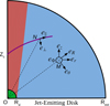 |
Fig. 1. Sketch of our computational domain. The central object and its interaction with the innermost disk are located below the inner boundary at Rd (green region), the near-Keplerian jet-emitting disk (JED) being established from Rd to the end of the domain Rext. An axial outflow (the spine) is emitted from the central regions (in red) and the jet is emitted from the JED (in blue). The solid purple line represents a recollimation shock surface starting on the axis at a height Zc. For each point N lying on this surface, we use local poloidal unit vectors (e⊥, e∥), respectively perpendicular and parallel to the shock surface. Also, at any point M inside the domain, we either use spherical (eR,eθ,eϕ) or cylindrical (er,eϕ,ez) coordinates. |
We further assume that a large-scale magnetic field is threading both the disk and the central object. The existence of this field allows the production of two outflows, one from the disk (blue region in Fig. 1) and one from the central spherical region (red region in Fig. 1). Hereafter, we always refer to the disk-emitted outflow as the “jet”, and to the outflow emitted from the spherical region (green zone in Fig. 1) as the “spine”. As our goal is to focus on the dynamics of the jet itself, we try to limit the influence of the spine as much as possible.
Two systems of coordinates centered on the mass M are used, spherical (R, θ, ϕ) and cylindrical (r, ϕ, z). Both the spine and the jet are assumed to be in ideal MHD and we numerically solve the usual set of MHD equations. This includes mass conservation
where ρ is the density and u the flow velocity, and the momentum equation is
![$$ \begin{aligned} \frac{\partial \rho \boldsymbol{u}}{\partial t} + \nabla \cdot \left[ \rho \boldsymbol{u}\boldsymbol{u} + \left( P + \frac{\boldsymbol{B}\cdot \boldsymbol{B} }{2\mu _o}\right) - \frac{\boldsymbol{B}\boldsymbol{B}}{\mu _o} \right] =- \rho \nabla \Phi _G ,\end{aligned} $$](/articles/aa/full_html/2023/01/aa44311-22/aa44311-22-eq2.gif)
where P is the thermal pressure, B the magnetic field, and ΦG = −GM/R the gravitational potential due to the central mass.
The evolution of the magnetic field is determined by the induction equation,
As we focus on highly supersonic flows, we decided to derive the pressure P and internal energy by solving the entropy equation,
where S = P/ρΓ is the specific entropy and Γ = 1.25 is the polytropic index (the same for all our simulations). This simple advection equation guarantees that the pressure does not assume nonphysical (e.g., negative) values. But on the other hand, it does fail to provide the correct entropy jump in the shocks. However, as long as the thermal energy of the flow remains negligible compared to the kinetic and magnetic energy, this should not present a problem.
Thanks to axisymmetry, the poloidal magnetic field can be computed using the magnetic flux function Ψ (which corresponds to R sin θ Aϕ, where A is the vector potential),
which already verifies ∇ ⋅ B = 0. An axisymmetric magnetized jet can therefore be seen as a bunch of poloidal magnetic surfaces defined by Ψ(R, θ) = constant, nested around each other and anchored on the disk for the jet and in the central object for the spine.
In steady state, Eqs. (1) to (4) lead to the existence of the following five MHD invariants, namely quantities that remain constant along each magnetic surface (Weber & Davis 1967):
-
the mass flux to magnetic flux ratio η(Ψ) = μoρup/Bp,
-
the rotation rate of the magnetic surface Ω*(Ψ) = Ω − ηBϕ/(μ0ρr),
-
the total specific angular momentum carried away by that surface L(Ψ) = Ωr2 − rBϕ/η,
-
the Bernoulli invariant
 ,
, -
the specific entropy S(Ψ) = P/ρΓ,
where Ω = uϕ/r and  is the specific enthalpy. We make use of these relations when designing boundary conditions.
2.2. Numerical setup
We solve the above set of equations using the MHD code PLUTO1 (Mignone et al. 2007). We configured PLUTO to use a second-order linear spatial reconstruction with a monotonized-centered limiter on all the variables. This method provides the steeper linear reconstruction compatible with the stability requirements of the scheme. A flatter and more diffusive linear reconstruction is employed in a few cells around the rotation axis to dampen numerical spurious effects that typically appear in these zones due to the discretization of the equations around the geometrical singularity of the axis. The HLLD Riemann solver of Miyoshi & Kusano (2005) is employed to compute the intercell fluxes. This solver is one of the best suited to properly capture Alfvén waves, a crucial element in properly modeling trans-Alfvénic flows. So as to match the order of the spatial reconstruction, we chose a second-order Runge-Kutta scheme to advance the equations in time. The ∇ ⋅ B = 0 condition is ensured by employing a constrained transport (CT) scheme, enforcing that constraint at machine accuracy.
The two-dimensional computational domain is discretized using spherical coordinates (R, θ) assuming axisymmetry around the rotation axis of the disk. The domain encompasses a spherical sector going from the polar axis (θ = 0) to the surface of the disk that is assumed to be θ = π/2 for simplicity, and is resolved with Nθ = 266 points in the θ direction. The cell size in the θ direction is mostly uniform, but decreases on a few cells near the axis. This is essential to our setup, as the expected collimation shocks are formed near the axis: an overly low resolution in this zone would prevent their formation. In the radial direction, the grid goes from Rd to Rext = 5650.4Rd with NR = 1408 points in a logarithmic spacing (ΔR ∝ R) so as to make sure the cells remain approximately square (ΔR ≈ RΔθ) far from the axis.
We choose such a huge numerical domain because our goal is to capture the recollimation shocks predicted in the self-similar solutions of F97. According to their Fig. 6, those shocks may occur at altitudes spanning from several hundred to a thousand times the jet launching radius. Our spherical grid with a ratio of 5650.4 therefore provides a suitable range to observe such shocks. The drawback of these huge spatial scales is of course the terrible contrast in timescales. The Keplerian time scaling in r3/2 means that in order to compute a full orbit at the outer disk edge, the inner one should have completed over 4 × 10⁵ orbits. This would be barely affordable if we were to use a standard evolutionary scheme. In order to achieve such long timescales, we designed a specific method that accelerates the numerical integration using larger and larger time steps to evolve the equations as the solution starts to converge towards a steady-state. This method is very successful and allowed us to significantly boost the evolution of our jets (see Appendix A).
2.3. Initial conditions
Our initial magnetic field is assumed to be potential, which leads to a second-order partial differential equation on Ψ(R, θ). In order to represent suitable self-similar solutions, we solve this equation by assuming
where the function Φ(θ) has been determined assuming that the initial field is potential, that is, current-free and force-free (Jϕ = 0).
The exponent α is a free parameter of the model leading to BR ∝ Bθ ∝ Rα − 2. For α = 0, field lines are conical, for α = 1 they are parabolic, and α = 2 describes a constant (straight) vertical field. The seminal BP82 solution is for α = 3/4.
As the magnetic field is potential, no magnetic force is initially imposed on the plasma. It is therefore assumed to be in spherically symmetric hydrostatic equilibrium (u = 0) with dP/dR = −ρGM/R2. We choose the following trivial solution:
The sound speed Cs is defined as  . In the following, ρa refers to the density at the axis immediately above the central sphere.
2.4. Boundary conditions
Boundary conditions must be imposed at the polar axis (θ = 0, R from Rd to Rext), at the outer frontier (R = Rext, θ from 0 to π/2), at the JED surface (θ = π/2, R from Rd to Rext), and at the spine boundary (R = Rd, θ from 0 to π/2). On the polar axis, usual proper reflecting boundary conditions are imposed on all quantities. The special treatment done for the other three boundaries is described, especially for the JED and spine boundaries where mass is being injected.
2.4.1. Outer boundary (R = Rext)
“Outflow” conditions are imposed at the outer frontier: for ρ, P, BR, Bθ, RBϕ, uR, uθ and uϕ, the gradient along the radial direction is conserved, and we use the Van Leer slope limiter to avoid spurious oscillations. Additionally, we enforce a positive toroidal Lorentz force on the subalfvénic part of this boundary.
2.4.2. Jet generation: the jet-emitting disk (θ = π/2)
We need to specify eight quantities (ρ, u, B, P) that must be representative of the fields expected at the surface of a JED. As the lifted material gets accelerated along a field line, its poloidal velocity will become larger than the slow magnetosonic Vsm, poloidal Alfvén VAp, and fast magnetosonic Vfm phase speeds. Crossing each of these critical speeds defines a regularity condition that determines one quantity at the jet basis, therefore leaving five free functions to be specified. However, we wish to control the mass loss from the JED, which requires that the injected outflow be already super-slow magnetosonic (hereafter super-SM). We therefore have to impose six functions at the JED boundary, leaving two free to adjust over time, Bϕ and BR, the latter controlling the magnetic field bending.
Our choice of boundary conditions at θ = π/2 (so that R = r) is therefore as follows:
where Ω* is the angular velocity of the magnetic surfaces (an MHD invariant in steady-state). We assume  , in agreement with a near Keplerian accretion disk, leaving four normalizing quantities, ρd, Csd, Bd, and ud, to be specified at Rd. These distributions are consistent with a self-similar JED and describe an ideal steady MHD flow with up ∥ Bp2, anchored on a disk that imposes magnetic field lines rotating at the Keplerian angular velocity ΩK. We note that the fixed component of the magnetic field threading the disk (Bθ) is actually the initial condition to conserve the magnetic flux injected into the computational domain, and only BR is allowed to vary in response to the jet dynamics.
In order to pick up values at Rd that are consistent with the jet calculations performed by BP82 or F97, we express the JED boundary conditions as a function of four dimensionless parameters: (1) the jet density ρd is fixed with respect to the density at the polar axis using ρd = δρa; (2) the disk sound speed (temperature) is defined relative to the Keplerian speed with ϵ = Csd/VKd; (3) the magnetic field strength Bd is controlled by measuring the θ component of the poloidal Aflvén speed with respect to the Keplerian speed, namely  ; and (4) the (vertical) injection velocity ud can be determined with the well-known mass-loading parameter κ introduced by BP82 using
By fixing ud/VKd = 0.1 for all the simulations, we obtain κ = 0.1/μ2. In order to be able to fix the value of the injection speed ud and therefore the JED mass flux, we must require that up > Vsm. As we are mostly interested in producing cold MHD outflows, we assume ϵ = 0.01 so that the θ component of the sonic Mach number is Msθ = ud/Cs = ud/VKdϵ = 10. As the total poloidal speed at the jet boundary is larger than ud, the sonic Mach number Ms = up/Cs > 10. As the poloidal Alfvén speed at the disk surface is much larger than the sound speed, Cs > Vsm and Ms > 1 is enough to warrant a super-SM condition.
We decided to vary the mass load and the disk Alfvén speed by only changing the disk density ρd (and keeping the injection speed ud and the disk magnetic field Bd constant for all the simulations). As a consequence, the density contrast δ can be expressed as a function of μ (or κ). We assume the relation δ = 100/μ2 = 1000κ. We highlight the fact that with our parametrization the JED boundary conditions are determined by only one dimensionless parameter, typically κ, while the other two free parameters μ and δ are determined as a function of κ, and ϵ is fixed for all the simulations.
2.4.3. Spine generation: the central object (R = Rd)
In the spine, we follow a similar methodology to that in the JED and specify six quantities along the inner spherical boundary at Rd. This again leaves two quantities that are free to evolve, Bϕ and Bθ. In order to conserve the magnetic flux injected into the computational domain, we fix BR(θ) to its initial value. We note that, as the Bθ(R) profile is fixed along the JED boundary (θ = π/2) and BR(θ) is kept constant in time along the spine boundary (R = Rd), the total poloidal field and its inclination BR/Bθ do not change with time at the inner radius of the disk (R = Rd, θ = π/2). The strength of the magnetic field is already determined by the value of μ chosen in the JED. As the outflowing material leaving the central region is in ideal MHD and we are looking for a steady jet, one has uθ = uRBθ/BR. This leaves us with the four distributions ρ, Cs, uR, and uϕ to be specified along θ.
If the central object possesses its own magnetosphere, then Rd might be considered as the disk truncation radius. What would be encapsulated within Rd could then be a complex combination of a stellar wind plus any type of magnetospheric wind (steady or not; see for instance Zanni & Ferreira 2013 and references therein). If the central object is instead a black hole, then Rd might be considered as the innermost stable circular orbit and what is hidden inside Rd would highly depend on the black hole spin. While a nonrotating black hole would provide no outflow, a rather strong magnetic flux concentration is seen to occur in GRMHD simulations of spinning black holes, leading to the generation of powerful outflows through the Blandford-Znajek process (see e.g., Blandford & Znajek 1977; Tchekhovskoy et al. 2010; Liska et al. 2018 and references therein).
However, our goal is to study the outcome of the jet emitted from the disk. We therefore decided to minimize the influence of the spine as much as possible. This was found to be an almost impossible task; details are given below. As pointed out in early works on magnetized rotating objects (e.g., Ferreira & Pelletier 1995), the jet power depends on the available electromotive force (emf) e = ∫Em ⋅ dl = ∫(u × Bp)⋅dl. While the disk provides an emf edisk ≃ ∫ΩKrBzdr, the central region provides eobj ≃ ∫ΩrBRRddθ. An obvious way to decrease eobj is therefore to allow Ω to decrease as one goes from the disk to the pole. We therefore use (in agreement with steady-state ideal MHD) uϕ = Ω*r + uRBϕ/BR, with magnetic surfaces rotating as

where f(θ) is a spline function varying smoothly from zero at θ = 0 to unity θ = π/2 (see Appendix B). Most of the simulations presented in this paper were done with Ωa = 0 (but not all, see Sect. 4.3). This choice is consistent with a nonrotating black hole but also with an innermost disk radius (our Rd) well below the co-rotation radius in the case of a star.
The fixed radial speed is defined through the sonic Mach number MsR, by uR = MsRCs. For MsR we assume a constant value along θ that can be derived from the JED boundary conditions by assuming its continuity at the inner disk radius Rd, MsR = Msθ|BR/Bθ|d = 10|BR/Bθ|d > 1. As the field inclination at the inner disk radius |BR/Bθ|d is constant, also MsR does not change with time. The sound speed at the base of the spine is computed as

where the sound speed on the axis Csa is computed so as to verify the Bernoulli integral Ea = E(θ = 0) at the axis. As the MHD contribution vanishes on the axis, one directly obtains
and
where uRa is the injection radial speed on the axis and ea = EaRd/GM is the Bernoulli integral normalized to the gravitational energy at Rd and will be used as a parameter to fix the axial spine temperature. We note that the normalized Bernoulli integral for the jet at Rd writes ed = λd − 3/2 + ϵ2/(Γ − 1), where  is the magnetic lever arm parameter, measured here at the anchoring radius ro = Rd. As our jets are cold, enthalpy plays no role and ed is mostly determined by λ (which is known only once the simulation has converged to a steady state). For our simulations, we expect a λ of around 10 (see our parameter space Fig. 15). We therefore fix ea = 2 in order to obtain a spine with a smaller energetic content than the surrounding jet. We note that, with our choice of parameters, the injection speed along the axis, set in Eq. (13), is higher than the escape speed. As the flow is cold and there is no magneto-centrifugal acceleration along the symmetry axis, the flow will gradually slow down along R in the spine from this very high speed in its core. The spine flow can cross the Alfvén and fast-magnetosonic critical points due to a decrease of the magnetic field intensity, not thanks to a flow acceleration.
Finally, for the density, we need to smoothly connect its axial value ρa to the much larger value injected at the disk surface ρd. We choose to do this by computing ρ(θ) = ηBR/(μouR), with the MHD invariant η following

with ηa and ηd being fully determined (see Appendix B). This method ensures that the mass flux to magnetic flux ratio has a smooth variation from the disk to the axis. For numerical stability reasons, as the strongest magnetic field is on the axis, the density in the code is normalized to ρa, providing a dimensionless density at the axis of 1.
2.5. Summary of parameters and normalization
Each simulation is entirely determined by the following dimensionless parameters and quantities: the radial exponent of the magnetic field α; the Bernoulli parameter ea (equal to 2 for most cases) and the spine angular frequency on the axis Ωa (equal to 0 in most simulations); and the cold jet parameters: κ,  , δ = 1000κ, ϵ = 0.01.
With our choices, we ensure that the injected flow is everywhere super-SM and that the main emf is due the JED, which is magnetically launching a cold jet. The profiles of several quantities along the magnetic flux near the lower boundary (inner spherical boundary and disk) reached by our reference simulation K2 at the final time can be seen in Fig. B.1.
This leaves us with only two free parameters, α and κ. We do not explore their whole range here but keep them within the parameter space of jets from JEDs as obtained by F97 but also by the solutions of Contopoulos & Lovelace (1994) and the simulations of Ouyed & Pudritz (1997a). The radial exponent α is varied from 10/16 to 15/16. In a strict self-similarity, this exponent must be consistent with the underlying disk, namely α = (12 + 8ξ)/16, where ξ is the disk ejection efficiency defined with the disk accretion rate as Ṁa(r) ∝ rξ (Ferreira & Pelletier 1995). However, our simulations are not strictly self-similar because of the presence of the axis and its spine, and so we also explore a slightly smaller α than the fiducial BP82 value α = 12/16. As discussed further below, values of α ≥ 1 are numerically problematic. The mass load parameter κ is varied between 0.05 and 1, which is a range globally consistent with BP82 and F97 jets, both solutions leading to a flow recollimation toward the axis.
The MHD equations have been solved with PLUTO and the results will be presented in dimensionless units. Unless otherwise specified, lengths are given in units of Rd, velocities in units of  , time in units of Td = Rd/VKd, densities in units of ρa, magnetic fields in units of
  , mass fluxes in units of
  and powers in units of
  . In order to be more specific, we translate these quantities for the case of a young star, assuming a star of one solar mass with an innermost disk radius Rd = 0.1 au, namely
The list of all the simulations performed in this paper is provided in Table 1, with their input parameters α and κ and several quantities that are measured at the final stage tend of the simulation. As explained in Sect. 2.4.1, the values of μ and δ are dictated by the values of κ. As discussed below, all our simulations display several recollimation shocks. In the table, we provide only the altitude (measured at the axis) of the first main recollimation shock Zshock. As stationary jets require them to become super-Afvénic and super-fast magnetosonic (hereafter super-A and super-FM, respectively), we also display the colatitudes  and
and  of the intersection of the outer boundary Rext and the Alfvén and FM surfaces, respectively. The last super-FM magnetic surface (defining the jet) can then be followed down to the disk, allowing us to identify the largest anchoring radius ro,FM that we consider in the JED. This allows us to measure the mass flux emitted from the JED as
  and compare it with the mass loss emitted from the spine only
  . We also compute the power emanating from the jet
  and compare it to the power emanating from the spine
  .
.
Simulations presented in this paper.
Simulations K1 to A5 were performed with a nonrotating spine, namely Ωa = 0 and ea = 2. Our reference simulation K2 is extensively analyzed in the following section. This reference was repeated with a lower resolution in K2l –all other things being equal– to verify numerical convergence. Section 4 addresses the influence of κ (simulations K1 to K5) and α (simulations A1 to A5). In Sect. 4.3, the effect of a rotating spine (simulation SP) is briefly addressed.
3. The Blandford & Payne case
3.1. Overview
In this section, we discuss our reference simulation K2 performed for the BP82 α = 3/4 magnetic field distribution and a mass-loading parameter κ = 0.1. It was run up to tend = 6.5 105 Td and has reached a steady-state in a sizable fraction of our computational domain (a quarter of an orbit has been done at ro = Rext).
Figure 2 displays the final stage reached by K2 at tend. The black solid lines are the poloidal field lines, the dotted red line is the Alfvén surface (where the Alfvénic Mach number m = up/VAp is equal to unity) and the dashed red line is the FM surface (where the FM Mach number n = up/Vfm = 1). The left panel shows our simulation on the full computational domain, with a close-up view on the scale used by (Fendt 2006) in the right panel. The background color is the logarithm of n on the left and the logarithm of the density on the right. The last magnetic surface characterizing the super-FM jet is anchored at ro, FM = 323 in the JED, and the critical surfaces (A and FM) both achieve a conical shape over a sizable fraction of the domain, which is characteristic of a self-similar steady-state situation. Our spine also achieves super-FM speed at an altitude of z ∼ 260.
 |
Fig. 2. Snapshot at tend of our Blandford & Payne simulation K2. Left: global view with field lines anchored on the disk at ro = 3; 15; 40; 80; 160; 320; 600; 1000; 1500, where the background is the logarithm of the FM mach number n. Right: close-up view of the innermost regions, where the background is the logarithm of the density. In both panels, black solid lines are the poloidal magnetic surfaces, the yellow solid lines are isocontours of the poloidal electrical current, and the red dashed (resp. dotted) line is the FM (resp. Alfvén) critical surface. |
The poloidal velocity vectors can be seen in Fig. 3. The velocity decreases radially very rapidly, mirroring the injection conditions, going from 3.5 at the spine to 0.2 at the edge of the super-FM zone (in VKd units). The white lines show streamlines inside which 50%, 75%, and 100% (from left to right) of the total super-FM mass outflow (spine + jet) rate is being carried in. These lines are anchored in the disk at r0 = 10, ro = 66, and ro, FM = 323, respectively. As dṀ/dR = 2πRVz falls off very rapidly, this plot shows that even ejection from a very large radial domain may be observationally dominated by the innermost, highly collimated regions up to ro ∼ 10, with the outer “wide angle wind” probably remaining barely detectable.
 |
Fig. 3. Snapshot of our reference simulation K2 at tend. We use the same color coding as in Fig. 2, left. The black arrows show the poloidal velocity. The white lines are streamlines inside which (from left to right) 50%, 75%, and 100% of the super-FM (spine+jet) mass outflow rate is carried in. |
The yellow solid lines are isocontours of the poloidal electric current I = 2πrBϕ/μo. These contours are very useful as they allow us to grasp several important features of the simulation: (1) The typical butterfly shape of the initial accelerating closed electric circuit can be seen up to a spherical radius R ∼ 3000. (2) For disk radii ro ≳ 2000, the electric current flowing out of the disk reaches the outer boundary (most of it in the sub-A regime at high colatitudes) and re-enters in the jet at smaller colatitudes, in the super-FM regime. (3) More importantly, several current sheets can be clearly seen (as an accumulation of current lines), highlighting the existence of several standing (stationary) recollimation shocks. To our knowledge, this is the first time that simulations of super-FM jets exhibit the patterns predicted in analytical jet studies. Justifications for this assessment are provided in Sect. 5.2.
These shocks are best seen in Fig. 4, which presents a zoom onto the region of interest. Five shocks (highlighted in colors) can be seen starting near the polar axis, following approximately the expected shape of the MHD characteristics in self-similar jets (see Figs. 3 in Vlahakis et al. 2000; Ferreira & Casse 2004). They are located at Z1 = 1850, Z2 = 2000, Z3 = 2160, Z4 = 2372, and Z5 = 2634. Only two of these shocks span a significant lateral portion of the jet (those best seen also in the left panel in Fig. 2). The first one (in red) leaves the axis at an altitude Z1 = 1850 (labeled Zshock in Table 1) and stays within our domain, finally merging with the FM surface (red dashed curve) around (r = 2500, z = 3800). The second shock starts at Z5 and leaves the simulation domain at (r = 1800, z = 5200), and is therefore not fully captured by our simulation. For this reason, only the first shock is extensively described here.
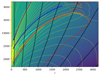 |
Fig. 4. Close-up view of our reference simulation K2 at tend showing the shock forming region, with field lines anchored at ro = 1.2; 2; 3; 4; 5; 7; 9. The five shocks are highlighted in red, orange, cyan, blue, and purple. We use the same color coding as in the left panel of Fig. 2. |
It can be seen that all shocks do occur only after the magnetic surface has started to bend toward the axis (with a decreasing cylindrical component Br), and give rise to a sudden outward refraction of the surface with its ouflowing material. This, plus the fact that their positions remain steady in time (see below), justifies our use of the name “standing recollimation shocks” to describe them. While these standing recollimation shocks appear quite generic for our set of simulations, we stress that fantastically large spatial and temporal scales are required to see them.
This simulation was also performed with a two-times-smaller resolution (see K2l in Table 1). We also observed standing recollimation shocks that are similar, although with less complexity.
3.2. Quasi steady-state jet and spine
Jet production is a very rapid process that scales with the local Keplerian timescale (especially As μ is constant with the radius). It is therefore an inside-out build-up of the jet with its associated electric circuit, until the innermost jet regions (including the spine) reach the outer boundary. This will take a time of typically text(ro = 1)∼Rext/Vz, with the maximal jet speed  . According to BP82, cold outflows with moderate inclinations and κ = 0.1 reach λ ∼ 10 (see their Fig. 2), which is exactly what we also obtain (see Fig. 15, with a minimum value λ = 11). This leads to a dynamical time text ∼ 1.3 × 10³ (in Td units) and so the innermost jet regions achieve an asymptotic state very early. However, the transverse (radial) equilibrium of the outflowing plasma is still slowly adjusting, because, as time increases, more and more of the outer magnetic surfaces achieve their asymptotic state, providing an outer pressure and modifying the global jet transverse equilibrium. This, in turn, necessarily modifies the shape of the magnetic surfaces as well as the associated poloidal electric circuit.
This means that the MHD invariants along each magnetic surface can always be defined (each surface is quasi-steady), but that they are also slowly evolving in time as the global magnetic structure evolves. For our simulation K2, the last super-FM magnetic surface is anchored at ro, FM = 323, defining a local Keplerian time TK = 5.8 × 10³. At that distance, the boundary is located at Zext ∼ Rext cos θFM ∼ 4430, leading to a dynamical time text(ro, FM)∼Zext/Vz(ro, FM)∼1.6 × 10⁴ (with λ = 14) as the speed distribution on the disk is Keplerian. We can therefore expect MHD invariants within our jet to evolve much less only after a time ∼104.
This slight evolution of the jet quantities over time is illustrated in Fig. 5. We chose to look at global quantities, such as the radius ro, FM of the last super-FM surface, the jet mass-loss rate Ṁjet, and the two colatitudes  and
and  that define the position of the two critical surfaces. We pick up their values at t = 5.1 × 10⁵ and plot their evolution by normalizing them to this “initial” value. It can be seen from Fig. 5 that their evolution is quite obvious: ro, FM keeps on increasing, leading to an increase in Ṁjet and a decrease in both
  and
and  . But the relative variations are less than 3% for ro, FM and 1% for the other quantities.
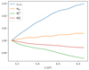 |
Fig. 5. Late evolution of several global jet quantities for the simulation K2: the radius ro, FM of the last super-FM surface, the jet mass-loss rate Ṁjet, and the two colatitudes |


We therefore consider that our simulation K2 has achieved a relatively global steady-state. In physical units (and for our choice of axial density ρa), the jet mass loss is about 2 × 10⁻⁷ M⊙ yr−1 with a magnetic field around 10 G at 0.1 au. The spine mass loss is only ∼10% of the jet mass loss, and so we can safely presume that the dynamics are mostly controlled by the JED, as expected. However, as the spine power is comparable to the jet power (Pspine/Pjet = 0.81), the impact of the spine on the collimation and topology of the electric field cannot be neglected. The influence of the spine is detailed in Sect. 4.3.
Figure 6 shows the various contributions to the Bernoulli integral E(ψ) along a magnetic surface anchored at ro = 100 at the final stage tend. It can be seen that E is indeed conserved and that jet acceleration follows the classical pattern (Casse & Ferreira 2000a): the kinetic energy (green) increases thanks to the magnetic acceleration, leading to a decrease in the magnetic contribution (magenta). Enthalpy (red) is negligible in this cold outflow. The presence of the shock is clearly seen around Z = 3800: the flow is suddenly slowed down and the energy is transferred back to the magnetic field, in agreement with the Rankine-Hugoniot jump conditions (see Appendix C). Beyond the shock, MHD acceleration is resumed but, at the edge of our domain, the magnetic field still maintains around 45% of the initial available energy.
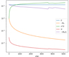 |
Fig. 6. Evolution of the various energy contributions along a magnetic surface of anchoring radius r0 = 100 for the simulation K2 at tend: the Bernoulli invariant E, the gravitational potential ΦG, the total specific kinetic energy u2/2, the enthalpy H, and the magnetic energy −Ω*rBΦ/η. The absicssa is the altitude Z(Ψ). |
The evolution along a magnetic surface of the five MHD invariants is shown in Fig. 7 for two surfaces, one anchored at ro = 100 (left) and the other at ro = 1000 (right). In order to plot η, Ω*, L, E, and S on the same figure, we normalize each quantity by its initial (at the disk surface) value at tend. On the left, variations of the invariants can indeed be seen but only at the shock located at Z = 3800; they remain very small, much less than 1% for all but the entropy (which is conserved to machine accuracy). On the right plot, the field line is anchored beyond ro, FM and the flow remains sub-FM while crossing no shock. Variations of the invariants are again observed, but always less than 0.3%. This shows that the PLUTO code is quite efficient and the MHD solution is indeed steady.
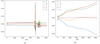 |
Fig. 7. Evolution of the MHD invariants along field lines of two different anchoring radii ro at tend for simulation K2. All invariants have been normalized to their values at ro. The absicssa is the altitude Z(Ψ). |
3.3. Jet collimation
Before analyzing the shocks in the following section, let us briefly discuss jet collimation. Figure 8 shows the initial magnetic field configuration (in dotted lines) along with the final configuration (solid lines) obtained at tend. Each color is associated with a different anchoring radius ro, allowing us to see the evolution from the initial potential field and the final full MHD solution. This plot clearly illustrates how magnetic collimation works. As the poloidal electric circuit responsible for the collimation must be closed, its sense of circulation must change within the whole outflow (defined as both the jet and its spine). The poloidal current density Jp is therefore downward in the inner regions and outward in the outer jet regions. As a consequence, field lines anchored up to ro ∼ 25 are focused to the polar axis (Z-pinch due a pole-ward Jp × Bϕ force as Jz < 0), while field lines anchored beyond ro ∼ 30 are de-collimated and pulled out (because of the outward action of the same Jp × Bϕ force as Jz > 0). See the right panel of Fig. 2 for the topology of J.
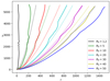 |
Fig. 8. Evolution of several magnetic field lines during the simulation computation, for different anchoring radii R0 and for the reference simulation K2. The field lines at the first output of the simulation (initial conditions) are shown in dotted lines. The field lines at the last output of the simulation (final state) are shown as full lines. |
The inner self-collimated jet region can only exist thanks to the existence of these outer jet regions that are pulled back and out. The final state of the jet collimation, namely the asymptotic jet radius achieved by these inner regions (the densest ones, possibly responsible for the observed astrophysical jets), is therefore also a consequence of the transverse equilibrium achieved by the outflow outskirts with the ambient medium. This balance is mathematically described by the Grad-Shafranov equation and expresses the action of the poloidal electric currents – how they are flowing and how electric circuits are closed within the jet – on the shape of the magnetic surfaces (Heyvaerts & Norman 1989, 2003a,b; F97; Okamoto 2001). We return to this point below.
3.4. Standing recollimation shocks
Our reference simulation K2 ends with five standing shocks, of which only the first (red in Fig. 4), starting on the axis around Z1 = 1850, is studied hereafter. This is for two reasons: (1) Contrary to the orange and cyan shocks, the red shock surface covers a large extension in the jet itself. It is therefore most probably related to the dynamics of our quasi self-similar jet, whereas these smaller shocks may be related to the spine–jet interaction. (2) It remains far away from the outer boundary (it ends up at the FM surface at a point r = 2500, z = 3800), which is clearly not the case for the purple shock and also probably not for the blue one.
3.4.1. Rankine-Hugoniot conditions
All shocks are due to the flow heading toward the axis (with decreasing, usually negative Br and ur components) at a super-FM velocity, resulting in a sudden jump in all flow quantities with an outward refraction of the magnetic surface (this can be seen in Fig. 8). The Rankine-Hugoniot jump conditions (see Appendix C for more details) are of course satisfied with the shock-capturing scheme of PLUTO and MHD invariants are conserved (up to some accuracy, as discussed above).
The left panel of Fig. 9 displays the evolution of several quantities along the red shock surface. It can be seen that the compression rate χ (green curve), defined as the ratio of the post-shock to the pre-shock densities, is larger than unity while remaining small (≤1.3, see red curve in the right panel), despite a very large Alfvénic Mach number m ∼ 100 (orange). This is probably because the shock is oblique and the incoming jet material does not reach very large super-FM Mach numbers n⊥ (defined as the ratio of the flow velocity normal to the shock surface to the FM phase speed in that same direction; blue curve). In fact, n⊥ ≤ n = up/Vfm, and at these distances the jet has reached its asymptotic state with a maximum velocity of  (VKo = Ω*ro the Keplerian speed at the anchoring radius). Assuming Bp ≪ |Bϕ|, m ≫ 1 and a jet widening such that r ≫ rA where rA is the Alfvén cylindrical radius along a flow line where m = 1, leads to
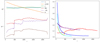 |
Fig. 9. Distributions along the shock of several quantities for K2 at tend. Left: normal incident FM Mach number n⊥, Alfvénic Mach number m, compression rate χ, relative variations of the toroidal magnetic field δBϕ and plasma angular velocity −δΩ, and total deviation δi (in rad) of the poloidal magnetic field line for the main recollimation shock. Right: compression rates χ of all shocks appearing in Fig. 4, using the same color code. The main shock corresponds to the red curve. See Appendix C for more details on this figure. |
which shows that the asymptotic FM Mach number critically depends on how much the jet widens (see Pelletier & Pudritz 1992 and Sect. 5 in F97). In our case, n ∼ 4 at the outer edge of the spine–jet interface, in agreement with self-similar studies. Following the main red shock along growing r, the incident angle3 of the magnetic field lines on the shock front decreases until turning into a normal shock on its external edge (r ∼ 2000). Hence, on this edge, the shock front coincides with the FM critical surface n = 1. As the shock becomes normal, n⊥ → n = 1 and the shock vanishes, with a compression rate χ going to 1.
The three other curves in the left panel of Fig. 9 describe other modifications in jet dynamics. The brown curve is the magnetic field line deviation at the shock front, δi = i2 − i1, where i is the flow incidence angle to the normal to the shock surface (subscripts 1 and 2 refer to the pre- and post-shock zones, respectively). The maximum deviation of 0.07 rad = 4° is very small, in agreement with the small compression rate.
The purple curve describes the relative variation of the flow rotation δΩ = (Ω2 − Ω1)/Ω1, which is always negative. The shock introduces a sudden brake in the azimuthal speed, meaning that the compressed shocked material is always rotating less. As t.e detection of rotation signatures in YSO jets is an important tool for retrieving fundamental jet properties (see e.g., Anderson et al. 2003; Ferreira et al. 2006; Louvet et al. 2018; Tabone et al. 2020), recollimation shocks appear to be a very interesting means to lower the jet apparent rotation. However, the rather weak shock found here only introduces a decrease of ∼20% at the outer edge of the shock.
The plasma loss of its angular momentum at the shock is of course compensated for by a gain of magnetic field (the angular moment is a MHD invariant). This means that the magnetic field lines are more twisted after the shock than before, as illustrated in the red curve showing δBϕ = (Bϕ2 − Bϕ1)/Bϕ1 > 0. The shock surface acts therefore as a current sheet with an electric current density flowing outwardly (in the spherical R direction).
3.4.2. Two families of shocks
The right panel of Fig. 9 displays the compression rate χ for the five shocks seen in Fig. 2, using the same color code. All shocks but the red one have larger compression factors near the axis. The orange and cyan shocks merge with the main red one (respectively at r ∼ 500 and r ∼ 900), leading to an increase in its compression rate χ. The large blue shock has the same behavior as the orange and cyan but remains alone (i.e., not merging with the red) with χ converging to 1, while the purple shock seems to have a similar behavior to the red one, maintaining a larger value for χ. Although these last two shocks are probably affected by their proximity with the outer boundary, it seems that two classes of recollimation shocks are at stake.
The first class (represented by the red and purple shocks) corresponds to the recollimation shock predicted in self-similar studies (FP97, Polko et al. 2010). The reason for their existence is the hoop-stress that becomes dominant as the jet widens, leading to a magnetic focusing toward the axis. As shown in FP97, such a situation always arises in the super-FM regime, meaning that a shock is the only possibility for the converging flow to bounce away. However, as long as no dissipation is introduced, such a situation will repeat. Indeed, after the flow refraction due to the shock, the magnetic field starts to accelerate the plasma again, the magnetic surface widens and the same situation repeats. One would therefore expect periodic oscillations and shocks on a vertical scale HR (measured on the axis). Figure 8 provides some evidence of this pattern for the field lines anchored at ro = 20, 30 or 40. The first recollimation shock (red) is quite far away from the disk (Zshock = 1850), but the second shock (purple) occurs at Z5 ≃ 2634. A much larger computational domain would be necessary in order to clearly assess a periodic pattern.
The second class of recollimation shocks (represented by the orange, cyan, and blue shocks) are limited to the vicinity of the spine–jet interface and are thereby a consequence of a radial equilibrium mismatch between these two super-FM outflows. The transverse equilibrium of a magnetic surface is provided by projecting the stationary momentum equation in the direction perpendicular to that surface, leading to the equation (FP97)

Here, ∇⊥ = e⊥ ⋅ ∇ provides the gradient perpendicular to a magnetic surface with e⊥ = ∇Ψ/|∇Ψ| and  , measures the local curvature radius ℛ of the magnetic surface. In the asymptotic region where these small recollimation shocks are observed, the field lines are almost vertical and gravity is negligible. The above equation therefore reduces to
Looking at Fig. 10, where the various forces are plotted as a function of the cylindrical radius at a constant height Z = 2400, it can be clearly seen that the dominant force is the hoop stress  (purple curve) near the spine-jet interface (dashed vertical line), defined as the magnetic field line anchored at ro = Rd. That pinching force overcomes the others (the above sum is actually nonzero and negative), indicating that the field lines do have a curvature and are actually converging toward the axis (therefore Eq. (18) is too simplistic). Nevertheless, this behavior of the forces is consistent with the stationary shape of the magnetic surfaces seen at Z = 2400 at those radii. Further out, downstream, the fifth (purple) shock will make the field lines bounce back again. This tells us that we are witnessing radial oscillations of the radius of the spine driven by a mismatch between the dominant forces (hoop stress, magnetic pressure, and centrifugal term).
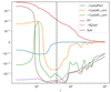 |
Fig. 10. Radial distribution of the radial accelerations and their sum at the altitude Z = 2400 for the simulation K2 at tend. The vertical dashed line corresponds to the spine–jet interface, namely the field line anchored at ro = Rd. |
This oscillatory behavior may be a generic feature of MHD outflows from a central rotator as shown by Vlahakis & Tsinganos (1997), because of the different scaling with the radius of the pinching force and the centrifugal force (as in the self-similar jet; F97). But it may also be triggered by the pinching due to the outer jet recollimation, namely the spine–jet interface response to the global jet recollimation. Indeed, no spine–jet shock is seen before the onset of the main recollimation shock. We further note that the five shocks are located at a slightly increasing distance from each other. Indeed, ΔZ12 = Z2 − Z1 = 150, ΔZ23 = 160, ΔZ34 = 212, and ΔZ45 = 262, which is the sign of some damping of the spatial oscillations at the spine–jet interface (see e.g., Vlahakis & Tsinganos 1997). This corresponds to three spine–jet shocks (orange, cyan, and blue) located between the two large jet recollimation shocks (red and purple), as can be seen in Fig. 4.
Despite the fact that the magnetic surfaces are in a steady state, it is useful to look at this spatial oscillatory pattern as the nonlinear outcome of transverse waves. Immediately after a shock, the flow is again outwardly accelerated leading to a widening of the magnetic surface and its refocusing toward the axis with the unavoidable shock. It will therefore take a time Δtz = ΔZ/uz to reach the next shock. On the other hand, any radial unbalance triggered immediately after the shock gives rise to a transverse (radial) FM wave that bounces back on a timescale of Δtr = 2r/Vfm measured at the spine–jet interface. In steady-state, these two times must be the same, which requires ΔZ ∼ 2nr, where n is the FM Mach number measured at the spine–jet interface. At Z = 2400, the width of the spine is r ≃ 40, and n ≃ 3, providing the correct order of magnitude for ΔZ ∼ 240. This is also verified for all other shocks. This correspondence strengthens the idea that these small shocks are actually triggered by the first large recollimation shock.
3.5. Electric circuits
The existence of these shocks drastically affects the poloidal electric circuits that go along with MHD acceleration (and of course collimation). This can be seen in Fig. 11, where several interesting circuits are shown in color. Each poloidal circuit corresponds to an isocontour of rBϕ, the arrows indicating their flowing direction.
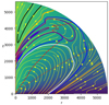 |
Fig. 11. Plot of the poloidal electric circuits at tend for simulation K2. The two red curves are the critical surfaces, Alfvén (dotted) and FM (dashed). The yellow curves are the poloidal electric circuits, defined as isocontours of rBϕ, where the arrow indicate the direction of the poloidal current density Jp. Four circuits are highlighted in particular: (1) the envelope of the inner accelerating current in white (rBϕ = −2.06), (2) the outermost circuit still fully enclosed within the domain in blue (Bϕ = −2.005), (3) a circuit closed outside the domain in orange (rBϕ = −1.80), and (4) a post-shock accelerating circuit in purple (also with rBϕ = −2.06). |
The white contour marks the last electric circuit that flows below the first recollimation shock and defines the envelope of the initial accelerating current. It links the disk emf with the accelerated jet plasma and flows back to the disk along the spine. This is due to the fact that the largest electric potential difference is with the axis.
The blue circuit is the last electric circuit fully enclosed within the computational domain. The current flows out of the disk (further away than the previous circuit) and makes a large loop that goes beyond (downstream) the main recollimation shock, flowing back on the axis below Z5 until it encounters the smaller shock at Z4 (blue curve in Fig. 4). As a shock behaves as an emf, with an outwardly (positive Jr) electric current flowing along its surface, the blue electric current gets around it and goes back to the axis where it meets the next shock surface at Z3 (cyan in Fig. 4). As that shock merges with the main recollimation shock, the blue electric current flows along these two surfaces, gets around the main shock (near the point r ∼ z ∼ 3000 in Fig. 11) and returns back to the disk via the spine, where it joins the white circuit below Z1.
As mentioned above, the outflowing plasma gets re-accelerated after each shock. This requires a local accelerating electric circuit, which is naturally enclosed within two recollimation shocks. One such circuit is exemplified by the purple contour in Fig. 11. It actually has the same rBϕ value as the white one, but is enclosed between the two large recollimation shocks. As the small shocks (orange and cyan in Fig. 4) merge with the main one, the purple accelerating circuit is the envelope of the current used to go from the first main shock to the second one flowing back to the spine just before Z5 (and getting around the shock starting at Z4 near the point r ∼ 2000, z ∼ 4000, like the previous blue electric circuit).
These three examples of electric circuits (white, purple, and even blue) are fully closed within the computational domain and therefore do not contribute to any further asymptotic collimation. However, it can be seen that the electric current outflowing from the disk beyond ro ∼ 2000 leaves the computational domain and is supposedly closed by the inflowing current that enters the computational domain at small colatitudes. One example of such an electric circuit is shown by the orange curve in Fig. 11. This inward electric current is responsible for the inner jet collimation at large distances, say at Z ≳ 3000, and is seen to flow back to the disk along the spine, which acts as a conductor. This implies that the asymptotic jet collimation is here somewhat controlled by an electric circuit that is not fully self-consistent. Indeed, this electric circuit is actually determined by the boundary conditions at Rext and there is no guarantee that its evolution is consistent with the disk emf. This is of course unavoidable but it may have an impact on the collimation properties of numerical jets (see discussion in Sect. 5). Moreover, as this current embraces very large spatial scales, very long timescales are consistently implied and may lead to evolution of the jet transverse equilibrium on those scales.
3.6. Time evolution
Figure 12 shows the evolution in time of the vertical height Z (measured at the axis) of all shocks found in the simulation. As discussed previously, it takes a time text(1)∼103 for the innermost jet (anchored at ro = Rd) to reach the boundary of our computational box. During this early evolution with t < text(1), the detected shocks correspond to the first bow shock where the jet front meets the initial unperturbed ambient medium. Once the jet has reached the boundary, the spine is in a steady-state while the jet transverse equilibrium continues to evolve due to the self-similar increase in its width. Indeed, the time to reach the outer boundary for a magnetic surface anchored at ro in the disk grows as  . It therefore takes a time ∼104 to achieve a steady ejection from ro = ro, FM = 323, where ro, FM is the maximum radius of the field lines that achieve a super-FM flow speed. The global jet structure is only expected to have a steady state beyond that time.
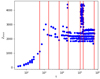 |
Fig. 12. Altitude Z of the different shocks (measured at the axis) as a function of time (in Td units) for simulation K2. The vertical lines correspond to the six times ti used in Fig. 13: t1 = 551, t2 = 2.08 × 10³, t3 = 8.51 × 10³, t4 = 1.99 × 10⁴, t5 = 1.05 × 10⁵, and t6 = 1.58 × 10⁵. The last vertical line is tend = 6.51 × 10⁵. |
The vertical lines in Fig. 12 trace six times t1 = 551, t2 = 2.08 × 10³, t3 = 8.51 × 10³, t4 = 1.99 × 10⁴, t5 = 1.05 × 10⁵, and t6 = 1.58 × 10⁵. The snapshots corresponding to each of these times are shown in Fig. 13, allowing us to see the global jet evolution. The times t1 and t2 have been chosen to enclose text(1). The bow shock with the ambient medium is clearly seen, as is the outward (radial) evolution of the jet width. At t2, several shocks near Z ∼ 2000 can be seen in both figures. The jet radial equilibrium is clearly not yet steady. However, Fig. 12 shows that while the positions of the shocks (as measured on the axis) are already close to their final values, their final number is not yet settled.
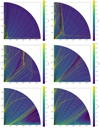 |
Fig. 13. Snapshots of our reference simulation K2 at different times (given in Td units). From top to bottom, left to right: t1 = 551, t2 = 2.08 × 10³, t3 = 8.51 × 10³, t4 = 1.99 × 10⁴, t5 = 1.05 × 10⁵, and t6 = 1.58 × 10⁵. The background color is the logarithm of the density, black lines are the magnetic surfaces, red lines the Alfvén (dotted) and FM (dashed) surfaces, and yellow curves are isocontours of the poloidal electric current. |
Four standing recollimation shocks seem to settle somewhere between t3 = 8.51 × 10³ and t4 = 1.99 × 10⁴, in agreement with our previous estimate; they can be clearly seen in Fig. 13, where some transient shocks located further up at Z > 4000 at t3 have disappeared at t4. Also, given the huge spatial scales involved, most of our JED is still evolving. For instance, while there have already been 3183 orbital periods at Rd at t4, the disk has done only half of an orbit at ro = 323. This can be seen in the shape of the FM surface, which has not yet reached its steady-state configuration (conical).
Beyond t4, the global flow is slowly evolving in time in some adiabatic way, with four standing recollimation shocks. The evolution of the jet outer regions and the progressive evolution of the A and FM surfaces to their conical shapes seems to produce no obvious evolution in the shocks until t5. At that time, a dramatic evolution is triggered with the appearance of shocks beyond Z4. Figure 12 clearly shows this pattern with the appearance of a fifth shock; its altitude Z5 evolves in time, consistently with Z4 until a steady-state is finally reached approximately near t6. Our final state tend shows no relevant difference in the positions of the five shocks. This evolution of the distribution of the shocks has only slightly affected the position of the farthest shock Z4, leading to the final regular distance ΔZ discussed above.
The appearance of a fifth shock at t5 leading – after a transient phase ending at t6 – to a new steady state jet configuration is illustrated in Fig. 14. The time evolution of the cylindrical radius of the field line anchored at ro = 3 (in blue) is measured at a constant height Z = 3500. It can be seen that this radius is steadily slowly decreasing in time, going from r ∼ 150 near t4 down to r ∼ 135 at t5 where some fluctuations are suddenly triggered. These oscillations describe a time-dependent behavior which ends at t6, with a new radial balance found at a smaller radius r ≃ 125. Globally, this evolution describes a magnetic surface that is first slowly getting more and more confined, and then enters an unstable situation until the formation of another (tighter) equilibrium. This behavior is consistent with the evolution of the electric current (red curve) that flows within that magnetic surface, which is seen to first steadily (although very slowly) increase until achieving a final value.
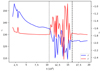 |
Fig. 14. Time evolution of the cylindrical radius r measured at Z = 3500 of the magnetic surface anchored at ro = 3 (blue curve) and the electric current I = rBϕ (red) flowing within that surface for simulation K2. The two vertical dashed lines correspond to t5 = 1.05 × 10⁵ and t6 = 1.58 × 10⁵. |
In these inner regions, transverse equilibrium of the cold jet is mostly achieved by the poloidal magnetic pressure balancing the toroidal pressure and hoop stress (see Eq. (18) and Fig. 10). In this Bennett relation, one gets
This relation shows that the toroidal field Bϕ is compelled to follow the same scaling as Bz in order to maintain the jet transverse equilibrium. If we assume that the self-similar radial scaling for the vertical field Bz is recovered at large distances, we get (rBϕ)2 ∝ r2(α − 1). As a consequence, for α < 1 (which is the case here), whenever the electric current is increasing, the radius of the magnetic surface decreases (as in a Z-pinch). This scaling provides ΔI/I = (α − 1)Δr/r = −0.25Δr/r, which is consistent with the evolution seen in Fig. 14.
This slow increase in time of the electric current flowing near the axis is a natural consequence of the increase of the disk emf edisk as the outer disk regions achieve a steady state. Indeed,  increases with rmax, which is the maximal radius in the disk that achieved a steady state. This increase in the available current is expected to stop when no further relevant emf is added. The available current is determined at the disk surface by the crossing of the Alfvén critical point, because it is that point that fixes the available total specific angular momentum carried away. One can therefore estimate the time where the current should level off as the time when the outermost magnetic field line reached the Alfvén point. Figure 14 shows that this is achieved approximatively around t6 with rmax ∼ 103, corresponding to a full orbital period at rmax equal to
  (we note that the time for the flow ejected at rmax to reach the outer boundary is comparable). After a time of a few 105 Td, our simulation has finally achieved a global steady state.
4. Parameter dependence
In the previous section, we showed that our reference simulation K2 behaves qualitatively like the self-similar analytical calculations of Blandford & Payne (1982) and F97, with a refocusing toward the axis and the formation of a recollimation shock. However, the presence of the axial spine breaks down the self-similarity and introduces additional shocks localized at the spine–jet interface.
To further understand the behavior of these shocks, we conducted a parameter study in κ and α, the jet mass load and the radial exponent of the disk magnetic flux, respectively. We finally ran one simulation with the same JED parameters as in our reference simulation K2, but with a rotating spine. All our simulations are presented in Table 1.
4.1. Influence of the mass loading parameter κ
In this section, we present our simulations K1 to K5, obtained with the same parameters as K2 except for the mass load κ which is varied from κ = 0.05 to κ = 1. Our parameter range in κ is slightly smaller than the one achieved by Blandford & Payne (1982) which goes down to κ = 0.01. It can be seen in Fig. 15, which represents the magnetic lever arm λ as a function of the mass-loading parameter κ. Each simulation is obtained for a unique value of κ but as the simulation is not strictly self-similar, we obtain a range in λ: the larger the anchoring radius, the larger the field line inclination at the disk surface and the larger the magnetic lever arm λ. To ease the comparison with Fig. 2 of Blandford & Payne (1982), for each simulation, we computed the anchoring radius ro at which the field line inclination  at the disk surface is equal to 1.4, 1.5, and 1.65. This allowed us to draw in our Fig. 15 iso-contours of
  , which are in agreement with the above expectations and analytical self-similar calculations (see also Fig. 3 in F97).
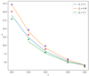 |
Fig. 15. Jet parameter space λ(κ) at the final stage of our simulations K1–K5 with α = 3/4. Each simulation is obtained for a unique mass loading κ and gives rise to a distribution of the magnetic lever arm λ with the radius: green, red, and blue dots correspond to anchoring radii ro = 5, 50, and 500, respectively. The solid curves are obtained for constant values (indicated in the panel) of the initial magnetic field inclination |

All simulations achieve a steady-state and exhibit roughly the same behavior as K2, as can be seen in Fig. 16. From top to bottom, κ increases from 0.05 to 1, the left panels showing the whole computational domain with the two critical surfaces in red (A, dotted and FM dashed) and the right panels providing a close up view around the shock-forming regions near the axis. Table 1 provides the value of several jet quantities: the spine mass-loss rate stays around 10% of the jet mass-loss rate, despite the net increase in Ṁjet (∝κ, factor 20 increase). Similarly, while the jet power Pjet scales in κ, the spine power stays around 80% of the jet power.
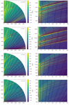 |
Fig. 16. Influence of the mass-loading parameter κ on the final stage of jets obtained with α = 3/4. The color background is the logarithm of the FM Mach number n, black solid lines are field lines, yellow lines are isocontours of the electric current rBϕ and the red dashed (resp. dotted) curve is the FM (resp. Alfvén) critical surface. The left panels show the whole domain and the right panels a close-up view around the shock-formation regions. In the left panel, the field lines anchoring radii are ro = 3; 15; 40; 80; 160; 320; 600; 1000; 1500. In the right panel, the field lines anchoring radii are ro = 1.2; 2; 3; 4; 5; 7; 9; 11; 13; 15. |
The first observation is that the altitude of the main recollimation shock (the one merging with the FM surface) decreases globally with κ. This is quantitatively shown in Fig. 17, where Zshock moves from 2150 down to 700. The same evolution occurs for the altitude Ztip where the main shock merges with the FM surface. Globally, as κ increases, the whole jet structure decreases toward the disk.
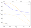 |
Fig. 17. Influence of κ (orange lines) and α (blue lines) on the altitude of the main recollimation shock. This is done by measuring two altitudes for each shock: its height at the axis (Zshock, solid lines) and the altitude of its outer edge (Ztip, dashed lines). The scale for κ is indicated below, while the scale for α is above. |
Such behavior is consistent with the self-similar calculations obtained by F97. Indeed, as evidenced in his Fig. 6, the denser the jet (larger κ), the sooner (smaller altitudes) recollimation takes place. This can be understood qualitatively by the fact that λ = 1 + q/κ, where q = |Bϕ/Bz| is the magnetic shear at the disk surface (F97). Now, as the mass load κ increases, the magnetic lever arm λ must decrease (see also Fig. 15). This translates into magnetic surfaces that open less, a less efficient magneto-centrifugal acceleration, and recollimation shocks that are not only closer to the disk but also show a smaller compression rate χ due to a smaller FM Mach number n.
However, the physical scales implied are very different. Here, a factor 20 difference in κ leads to a decrease in Zshock by a mere factor 3, with a minimum value of 700. In F97, the mass-loading parameter κ ∼ ξ varies from 0.01 to 0.05 only (for a constant disk aspect ratio, see his Fig. 3) but leads to variations in recollimation altitudes that span six decades. Our lowest Zshock obtained for κ = 1 is still much farther away than the minimum height of ∼10 found for κ ∼ 0.05 in F97.
This discrepancy can of course be attributed to the very different injection properties. Indeed, our numerical simulations assume a supersonic flow while the self-similar calculations compute the disk structure and outflows are found to only be super-SM (and still subsonic) at the disk surface. However, our guess is that the huge difference in the shock position is probably due to the existence of the spine, which breaks down the self-similarity. Indeed, recollimation is due to the dominant hoop stress, and while in our case all quantities are leveling off on the axis, strictly self-similar solutions have an axial electric current that grows without limits. For instance, at a cylindrical distance r = 0.1 from the axis at the spine basis, our Bz remains comparable to the disk field, Bϕ goes to zero, and the normalized Bernoulli integral e has decreased by a factor 5 (see Fig. B.1). Self-similar solutions, on the contrary, have fields and a Bernoulli integral increasing respectively by a factor 105/4 = 17.8 and 10. This suggests that the conditions assumed on the axis most certainly affect the overall jet collimation properties. We return to this aspect later on by changing the spine properties.
A second interesting aspect is the appearance of a second ensemble of shocks arriving at higher altitudes, namely Z > 3000 for κ = 0.5 and Z > 2000 for κ = 1. This second group of shocks is also composed of two large recollimation shocks separated by smaller ones. The distance (measured at the axis) between the two large shocks is comparable to the width of the first group of shocks. As discussed in Sect. 3.3, this hints to the fact that each group is caused by the global jet recollimation dynamics, which should be periodic in the Z-direction on a scale HR. Looking at the simulation K4 with κ = 0.5, this would give HR ∼ 1650, while the width of each group is around W ∼ 300 (the first group of shocks being located between 1150 and 1450, and the second between 3100 and 3400). As long as no dissipation is introduced, such a periodic behavior should continue in a box of infinite size.
4.2. Influence of the magnetic field distribution α
In this section, we vary the magnetic flux distribution exponent α in our simulations A1 to A5, keeping all other parameters (see Table 1) constant. A strict mathematical self-similarity links the magnetic field distribution α with the disk density in such a way that α = (12 + 8ξ)/16, where ξ is the disk ejection efficiency and is related to the disk accretion rate Ṁa(r) ∝ rξ (Ferreira & Pelletier 1995). As long as material is only outflowing from the disk (namely ξ > 0) and jet power is only released from accretion (namely ξ < 1, F97), this leads to the unavoidable constraint 12/16 < α < 20/16.
Only α = 12/16 can be compared to the cold jet solutions of F97, assuming an ejection efficiency ξ < 0.1. Larger values of α > 12/16 would require a disk ejection efficiency of ξ = 0.125 up to 0.5. These values are only achievable in analytical studies by introducing an additional heat deposition at the disk surface (magneto-thermal flows, Casse & Ferreira 2000b) and/or a much smaller magnetic field strength (Jacquemin-Ide et al. 2019). However, the physical processes required to get these solutions are missing in our simulation setup. We nevertheless vary α in order to allow a comparison with the self-similar jet solutions found by Contopoulos & Lovelace (1994), who tested the effects of α ranging from 0.5 to 1.02. We did not succeed to numerically obtain steady-state solutions for α ≥ 1 for reasons that are discussed below, and show only simulations with α ranging from 10/16 = 0.625 to 15/16 = 0.937.
All our A1 to A5 simulations reach a steady state with the same overall behavior as K2, namely the existence of two main recollimation shocks within the computational domain, separated by several smaller standing shocks located at the spine–jet interface. This can be clearly seen in Fig. 18 where, on the other hand, a trend with α can be observed. Indeed, the radial extension of the shocks decreases with α. This can also be seen in Fig. 17 which shows that the altitude Ztip of the main recollimation shock decreases with α, while its altitude Zshock at the axis barely changes. For simulations A1 (α = 10/16) and A2 (α = 11/16), the main recollimation shock ends out of the box, and therefore Ztip cannot be defined. However, the value of Zshock remains similar (see Table 1). This is a geometrical effect due to the fact that, as α increases, the magnetic field configuration goes from a highly inclined magnetic configuration (α = 0 corresponds to a monopole) to one that is much less inclined (α = 2 is a purely vertical field). This can be seen in the shape of the magnetic field lines (black solid lines) in Fig. 18. This geometrical effect translates into a smaller incidence angle near the axis and therefore to weaker shocks (the incidence becomes normal and n⊥ decreases to unity).
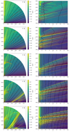 |
Fig. 18. Influence of the magnetic field distribution α on the final stage of jets obtained with κ = 0.1. We use the same notations, colors, and field lines anchoring radii as in Fig. 13. |
For α = 10/16 and 11/16, the shocks still exist but the MHD characteristics are much more vertical than in K2. A larger box would probably be necessary to recover the K2 behavior. The opposite trend can be seen for α = 14/16, with less vertical MHD characteristics allowing now the second main recollimation shock to merge with the FM surface within the domain.
Table 1 also shows that as α increases, the last radius on the disk giving rise to a super-FM flow increases and the colatitudes (measured at the outer boundary)  and
and  of the critical FM and A surfaces decrease. These results are a natural consequence of the magnetic field distribution becoming more vertical as α increases. As the jet mass loss Ṁjet and jet power Pjet are computed up to r0,FM which increases with α, Ṁjet and Pjet increase with α. Still, the mass loss increases even when computing up to a fixed radius. Indeed, the density decreases less with an increasing α (ρ ∝ r2α − 3) and the outer disk regions contribute more to the mass flux and jet power. Moreover, as the distribution in density is flatter with an increasing α, it is only natural that Ṁspine/Ṁjet and Pspine/Pjet decrease when α increases.
In summary, we find that the altitude of the shocks barely changes with α, which is in strong contrast with Contopoulos & Lovelace (1994). Indeed, their Table 1 shows that as α increases from 0.5 to a critical value 0.856, their self-similar jet becomes super-FM and undergoes a recollimation at a distance that increases by several decades (as in F97). As discussed above, we believe that this discrepancy is due to our nonstrict self-similar scaling (which forbids the unlimited growth of the inner electric current and the subsequential Z-pinch in self-similar solutions) and the presence of the spine. Contopoulos & Lovelace (1994) also report that their solutions with α > 0.856 remain sub-FM, while we clearly achieve super-FM flows up to α = 0.937 = 15/16. This is again probably a difference in our jet radial balance, leading to a slightly different jet acceleration efficiency. Finally, their solutions with α = 1, 1.01, and 1.02 remain sub-FM but evolve through a series of radial oscillations at logarithmically equal distances in Z.
Our simulation A5 is the simulation with the largest value α = 15/16, of close to unity. Although the final integration time tend is quite comparable with the other simulations, its appearance clearly shows that the global configuration is still far from achieving a steady state like K2. This can be seen in Fig. 18, in the shape of the critical surfaces but also on the isocontours of the poloidal electric circuit (yellow curves) that are still struggling to find their final state. This is normal and points to a numerical difficulty in computing MHD codes when the magnetic configuration is such that α ≥ 1.
Indeed, it has been argued above that for self-similar boundary conditions, the jet transverse balance imposes a toroidal magnetic field scaling with the vertical magnetic field. This leads to an electric current at the disk surface behaving as I = rBϕ ∝ rα − 1. Magnetic configurations with α < 1 correspond to a poloidal current density leaving the disk surface and closing along or near the spine (where it flows back to the disk), whereas configurations with α > 1 correspond to an inward poloidal current density, with current closure being done only at the outskirts of the outflow (F97). As div J = 0 in ideal MHD, all electric circuits must be closed. Let us define a radius in the disk rI such that for r < rI, the electric current flows down into the disk whereas it flows out of it for r > rI. For α < 1, rI is always larger but close to Rd implying very short timescales. As discussed in Sect. 3.6, as time is evolved, the outer disk regions provide more current that struggles to reach the innermost disk radius. But a global radial balance can be achieved consistently with the electric current closure condition because the local time near rI is small. On the contrary, configurations with α > 1 have rI that is constantly increasing in time (as t2/3), leading to an electric circuit that freezes in time and therefore to a transverse MHD balance that takes a much longer time to achieve steady state. We observe this behavior for all values of α > 1 and none of these simulations has achieved a steady state.
The limiting value α = 1 (close to our A5 simulation) would correspond to rI = Rd and absolutely no electric current flowing out of the disk until some outer radius. Current closure could only be done through the spine and the outer jet interface with the ambient medium. But then, no magnetic acceleration would be possible as no electric current could be used along the magnetic surfaces. This would correspond to an exact force-free field configuration fully determined by the chosen boundary conditions. To compute such a situation, boundary conditions must be designed where the jet launching region has a finite extent. However, we doubt that the outcome would be a force-free field unless explicitly enforced. This is beyond the scope of this paper.
4.3. Influence of a rotating central object
In this section, we do not intend to fully explore the physical parameters of the spine but instead wish to probe whether the spine, despite its small spatial extent, has indeed a profound influence on the overall jet dynamics. All simulations K1-K5 and A1-A5 were done with the same nonrotating central object in order to minimize its emf and numerically follow the outcome of a jet emitted from an outer self-similar disk (see Sect. 2.4.2). Our choice of parameters gives rise to a spine carrying typically 10% of the mass flux, and therefore providing only a small contribution to the overall outflow. Nevertheless, this spine carries a large fraction of the emitted power, even superior to that of the disk for the simulation A1. The spine plays an important role in introducing extra standing shocks at its interface with the jet, but is probably also determining the altitude where the first large recollimation shock occurs. Indeed, as discussed in the previous sections, the amount of electric current that is flowing along the innermost axial regions (along the spine and the inner jet) is what determines the strength of the Z-pinch acting upon the jet and thereby the altitude Zshock.
In order to probe this idea, we ran another simulation with a rotating object (simulation SP in Table 1). We chose an object rotating at the same angular velocity as the innermost disk radius Rd, namely Ωa = ΩKd. This is for instance representative of a star–disk interaction where the disk truncation radius is located at the co-rotation radius. By doing so, the emf due to the central object becomes non-negligible and we expect a stronger poloidal electric current. However, care must be taken as enhancing the hoop stress may also lead to an overwhelming radial pinch. To prevent this and get somewhat closer to the self-similar conditions, we also increase the value of the Bernoulli integral on the axis and use ea = 10 (ea = 2 for the other simulations). We note that the Bernoulli invariant from the innermost disk region is ed ≃ λd − 3/2 ∼ 10. This translates mostly into a thermal pressure that is five times larger than previously. Thus, our new conditions for the spine provide a rotation and a specific energy that are only comparable to those at the inner jet, not much larger as in a self-similar situation.
Figure 19 shows the final outcome of this new simulation. It achieves a global steady state with the same features as in our reference simulation K2. However, the shocks are, as expected, localized at lower altitudes, allowing a second set of large recollimation shocks to appear near Z ∼ 3700. The first large recollimation shock appears at Zshock = 1300, which is significantly smaller than Zshock = 1850 obtained for a nonrotating central object. This result confirms the role of the central object in shaping, through its spine, the collimation properties of the jets emitted by the surrounding disk. This is very promising and deserves further investigation.
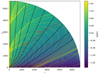 |
Fig. 19. Snapshot at tend of our SP simulation with a rotating spine, α = 3/4 and κ = 0.1. We use the same color coding as in Fig. 2. The magnetic field lines (black solid lines) are anchored at the same disk radii. |
5. Discussion
5.1. Caveats
This paper provides some novel information on the collimation of jets emitted from self-similar magnetized disks. However, we would like the reader to pay attention to several caveats:
As we tried to replicate a Blandford & Payne process, we mostly explored the ejection conditions on the disk and not on the source, with the exception of the rotation (see Sect. 4.3). For instance, we kept a value of sonic mach number MS = 10 on the whole ejection zone, thus only creating cold jets. It would be interesting to provide a real exploration of the spine parameters to better understand the role of the central object in the collimation.
The shocks displayed in our simulations are rather weak (χ ∼ 2 near the axis, χ ∼ 1.3 in the jet). This is probably due to our isentropic scheme, but as the simulations only reach small values of n, the compression rates are intrinsically low (see Appendix C). Moreover, as shown in Eq. (C.4) the impact of those shocks on jet angular velocity in YSOs is probably weak, at least for jets achieving m2 ≫ 1.
Our adiabatic solutions do not allow energy dissipation, and so the shocks should go on, one above the other, with each shock producing its own local accelerating circuit. This is showcased by the presence of a second subset of shocks in simulations K4, K5 (see Fig. 16), and SP (see Fig. 19). Thus, this setup does not allow the presence of a “true” asymptotic circuit that would extend up to infinity on the jet axis.
These simulations are highly dependent on the numerical setup. In order to capture the expected shocks, we used an HLLD solver, switching to a more diffusive HLL solver and MINMOD linear spatial reconstruction in regions of extremely low density and very high Alfvén speed. For the same reason, we used a higher resolution in θ around the axis to resolve the shocks. Still, we were only able to reach very long timescales thanks to a novel method that boosts the numerical integration (see Appendix A).
5.2. Comparison with other numerical works
In this section, we only compare our findings with previous 2D platform simulations of nonrelativistic jets. Indeed, relativistic jets develop an electric force that deeply affects the asymptotic collimation, forbidding a direct comparison with our nonrelativistic setup. We also disregard 3D jet simulations as they usually introduce a whole new phenomenology related to jet instabilities that are not present in our work. Making 3D simulations of our jets is planned for future work.
Platform simulations of jets have a great many degrees of freedom and it is therefore very difficult to determine the exact generic results on jet collimation that can be derived from them. Even if the whole injection domain is chosen to be sub-SM, three free distributions must be chosen at the boundary (assumed to be the disk surface), usually Bz(r),ρ(r), and uz(r). The disk being assumed to be Keplerian, most previous works used field lines rotating at Keplerian speeds and uz = VinjVK, where Vinj is a small dimensionless number. We use the following notations Bz ∝ rα − 2 and ρ ∝ r−αρ leading to
with ακ = −2αμ = −2α + αρ + 3 and the cylindrical radius is normalized to the inner radius Rd. For a given magnetic field distribution, the way the mass is injected in the outflow (or how the magnetic energy must vary within the disk) is an important quantity allowing to compare the various jet models. Our injection conditions (Eq. (8)) have αρ = 2α − 3, and therefore αμ = ακ = 0, which is in agreement with self-similar studies (BP82; F97). For our explored range in α < 1, our jets are always dominated by the mass flux emitted from the innermost disk regions. As discussed previously, the spatial and temporal scales are also very important in order to obtain recollimation shocks. We recall that our spherical domain goes up to Rext = 5650Rd covered with 266 × 1408 zones and lasts Tf ≳ 105 Td.
The box size and timescales achieved in the pioneering works of Ouyed & Pudritz (1997a,b, 1999) were of course quite small, with a cylindrical domain (z, r) = (80, 20) in Rd units and a resolution of (500, 200) cells, with the simulations lasting up to Tf ∼ 500. These authors studied mostly α = 1 and α = 2 magnetic configurations, assuming αρ = 3/2, μd = 0.01 and with no injected spine. Their jets have therefore a steeply decreasing κ (or increasing μ) with ακ = 3/2 − 2α, providing situations very different from ours. The authors argued that the nature of the outflow (steady or not) is mostly determined by the mass load κ, with unsteady jets containing shocks and associated knots arising at small values of κd ∼ 10−2. While these shocks are indeed due to jet material being focused toward the axis, Ouyed & Pudritz (1997a,b, 1999) did not report any steady-state situation. Our own simulations show that their timescales were still too short to warrant a transverse jet balance, especially for α ≥ 1. Moreover, it remains unclear as to whether these knots were indeed a consequence of a small mass load κd or due to the boundary conditions used at the jet basis, which were too numerous and therefore over-determined the outflow dynamics (see discussions in e.g., Bogovalov 1997; Krasnopolsky et al. 1999; Ramsey & Clarke 2019).
Ustyugova et al. (1999) showed that if the simulation region is elongated in the z-direction, then Mach cones may be partially directed inside the domain, leading to an artificial influence (usually collimation) on the flow. Using a domain (z, r) = (200, 170) with 100 × 100 cells, these authors showed that this effect can be reduced with a square or spherical grid.
Pudritz et al. (2006) extended their work by exploring a larger range in α = 1, 3/4, 1/2, 1/4, using κ = 5r3/2 − 2α, μd = 0.01 and no spine. These latter authors argued that the collimation of a jet depends on its radial current distribution, which in turn is prescribed by the mass load. Simulations with α = 1, 3/4 would collimate to cylinders due to a decreasing κ leading to a large Bϕ, whereas simulations with α = 1/2, 1/4 with an increasing κ would produce a smaller Bϕ and jets closer to wide-range outflows with parabolic collimation. However, our simulations show that the physical scales needed to observe the correct asymptotic state are much larger than those achieved in these early simulations. Moreover, it is indeed correct that self-collimation depends on Bϕ, which, in a magnetic jet that carries away the disk angular momentum, namely −rBϕ/η ∝ Ωr2, varies as Bϕ ∝ κ(r)Bz at the disk surface. In their case, this expression leads to Bϕ ∝ r−1/2 − α, which is indeed more steeply decreasing with α. (However, our guess is that the collimation observed within the box of Pudritz et al. 2006 is mostly a consequence of the potential magnetic field configuration used as the initial condition, as also illustrated in Fig. 8.) Therefore, the smaller α, the wider (less collimated at a fixed distance) the jet.
The influence of the magnetic field profile α on the asymptotic jet collimation has also been investigated: Fendt (2006) performed 40 simulations in a larger cylindrical grid (z, r) = (300, 150) with 256 × 256 cells, with the simulations lasting up to Tf ∼ 300 to 5 103 (for those achieving a steady state over at least 50% of the grid). He explored a wide range in αρ from 0.3 to 2 and in α from 0.5 to 1.8, using the same boundary conditions as Ouyed & Pudritz (1997b), with Vinj = 10−3, κd = 5, no spine, and μd varying between 0.1 and 2.67. Fendt (2006) confirmed that the degree of collimation is decreasing for a decreasing α regardless of αρ, in agreement with our suspicion that the overall MHD collimation trivially follows the potential field configuration (see also Sect. 3.2). For α > 1.6, no steady-state jet is actually found, with a wavy radial pattern evolving along the outflow. This is consistent with our finding that for α ≥ 1 the timescales for reaching stationarity become overwhelmingly long and also with the existence of radially oscillating, sub-FM analytical solutions for α ≥ 1 (Contopoulos & Lovelace 1994). Fendt (2006) also reports a degree of jet collimation increasing with the jet magnetization exponent, namely with μσ = −ακ − 3/2 (see his Eq. 10). Now, of the 40 simulations, only 6 have ακ = αμ = 0 and 8 have ακ > 0, meaning that most simulations describe a mass loading decreasing with the radius. None of the simulations show standing recollimation shocks, even in the BP82 case obtained with μd = 0.177 (we use μd = 1). Putting aside this difference, our Fig. 12 shows that around their final time Tf = 5000, we observed shocks only around Z ∼ 1900, far beyond their computational domain.
Krasnopolsky et al. (1999) used a cylindrical grid (z, r) = (80, 40) with 256 × 128 cells, with the simulations lasting up to Tf ∼ 170, introducing a ballistic axial flow below Rd (the spine), injected close to the escape speed and surrounded by a disk wind. These authors used the correct number of boundary conditions and, by testing the effects of adjusting the size of the box, they showed the drastic importance of the amount of magnetic flux becoming super-A within the box on the overall flow collimation. They studied mostly α = 1/2 and 3/4 with μd = 4 and rather flat density distributions leading to ακ > 0, from 2 to 3/2. The authors do not report any time-dependent behavior seen in previous studies, which they attribute to both the existence of their sub-FM inner spine (where magneto-centrifugal acceleration is inefficient) and the correct treatment of boundary conditions. This latter work was extended by Krasnopolsky et al. (2003) on a much larger box (z, r) = (103, 103) with 190 × 210 zones, with the simulations lasting an unspecified time Tf. They only studied the case α = 1/2, with ejection from a finite zone ro = Rd and ro = 10Rd, yielding αρ = 1 (ακ = 1) or αρ = 3 (ακ = −1). The authors found that the collimation degree of this finite jet is improved for a steeper density profile, namely with a decreasing mass load with the radius, as discussed above. Krasnopolsky et al. (2003) report neither recollimation toward the jet axis nor radial oscillations, and attributed this behavior to their nonself-similar scaling. Our own results show instead that recollimation should be seen farther out (beyond their box) and that radial oscillations are expected only for α > 1.
Using the same grid and numerical setup as Krasnopolsky et al. (2003), Anderson et al. (2005) studied the effect of κd on the collimation of a cold BP82 jet model with α = 3/4 and αρ = 3/2 (thus ακ = 0). These authors varied κd from 6.3 10−3 to 19 assuming that ejection takes place only from ro = Rd and ro = 10 Rd (but enforcing Bz to zero at the edge of the launching region), while we assumed ejection from the whole disk and varied κd only from 5 × 10⁻² to 1. Despite the truncation due to the limited ejection range and the (almost) purely radial magnetic field at the edge of the launching region, Anderson et al. (2005) recover the same results as in steady-state jet theory (FP97): jets become increasingly open as κd decreases (see discussion in Sect. 4.1). Anderson et al. (2005) do not report any recollimation shock (although wiggles can be seen in their Fig. 4) but again, our shocks fall below Z = 1000 (within their box) only for κd ∼ 1 (see Fig. 17). We conclude that their box was too small to observe any standing recollimation shock. The authors report the inability to reach steady state (the timescale Tf is unspecified) for κd larger than unity, when field lines start to oscillate and produce ripples that propagate outward. This behavior is consistent with analytical studies and is related to the capability to produce super-A flows when they are heavily loaded (or have a weak magnetic field). Indeed, magnetically driven cold flows are possible only up to κ ∼ 1, leading to a magnetic lever arm λ ∼ 2. For larger mass loads (and smaller λ), gravity plays an important role, with the Alfvén surface getting closer to the disk, requiring the field lines to be bent by much more than the fiducial 30° at the disk surface4 (see Fig. 4 and discussion around the Grad-Shafranov equation in Jacquemin-Ide et al. 2019).
The largest axisymmetric simulations have been provided by Ramsey & Clarke (2011, 2019), using nine levels of AMR in a cylindrical grid (z, r) = (8 × 10⁴, 5 × 10³)Rd with simulations lasting up to Tf ∼ 6 × 10⁴. These authors computed the propagation and evolution of eight jets up to observable scales, defined with varying mass loads κd from 5 × 10⁻² to 32 and αρ = 3/2, α = 1 (thus a decreasing mass load with ακ = −1/2). In the simulations of these latter authors, mass is injected with Vinj = 10−3 and there is no injected spine as in Ouyed & Pudritz (1997a), although a spine naturally emerges. In all simulations, Ramsey & Clarke (2011, 2019) observe that regions beyond ro ∼ 10 Rd fail to displace the hot atmosphere and that the outflow is stifled, despite the decrease in κ. This is actually consistent with our previous discussion for simulations with α ≥ 1, which take a much longer timescale to reach steady state. Nevertheless, as the inner parts of the outflow evolve on much shorter timescales, some quasi-stationary situation can settle (see their Sect. 5.3). With no surprise, this is the case for small mass loads, while knots appear for κd = 0.5 (simulation E) and are recurrent (quasi-periodic) for κd = 2. These knots are not to be compared with our standing recollimation shocks, as none of the MHD invariants are constant along field lines passing through them. They are made of plasmoids launched from Rd ≲ ro ≲ 2Rd, where gas is both dense and hot. The knot formation mechanism is here directly related to the jet-launching process from this innermost disk region. Indeed, in this region, the field line bending is insufficient to drive the massive injected material, until a sufficiently strong toroidal field builds up and lifts the matter, in agreement with steady-state theory of massive outflows (F97; Jacquemin-Ide et al. 2019). The regularity of knot spacing is indicative of a simple oscillator related to the necessary build up of a strong toroidal field. These plasmoids are magnetically confined by the surrounding poloidal magnetic field, follow the path of the jet, and eventually merge together. For larger mass loads (κd = 8 and 32, simulations G and H), the outflows are fully unsteady while keeping their global structure (probably because of their 2D nature, as destroying instabilities such as kink or Kelvin-Helmholtz require 3D, as argued by the authors).
To our knowledge, no previous jet simulation has shown the existence of standing recollimation shocks, either because the computational domain was too small and/or the simulation timescales were too short. These limitations are even worse of course for simulations that do take into account the disk physics, as they must also struggle to follow the disk and the mass-loading process.
The first of these simulations computed an accretion–ejection configuration with α = 3/4 and αρ = 3/2 (the BP82 case) within a cylindrical grid (z, r) = (80, 40) on a time Tf = 251 only (Casse & Keppens 2002, 2004). On these timescales, the mass-loading process is computed, leading to the inside-out establishment of self-similar conditions with ακ = 0. Further simulations, carried out with the same initial configuration but exploring various disk parameters, were computed on slightly extended scales, a grid (z, r) = (120, 40) on a timescale of Tf = 400 (Zanni et al. 2007; Tzeferacos et al. 2009, 2013) and a grid (z, r) = (180, 50) on a timescale of Tf = 5.6 × 10³ (Sheikhnezami et al. 2012). As most of these works were focused on the disk physics and less on the jet dynamics, they provided little information about the latter. The simulations of Stepanovs & Fendt (2016) were done on a spherical grid up to Rext = 1500 with (NR × Nθ) = (600 × 128) zones and up to Tf = 104, for the same BP82 initial configuration. Such scales would be relevant for the appearance of recollimation shocks but they only show close-up views below R = 30 and focus instead on the accrection–ejection correlations. However, the long timescales allow us to see a radial redistribution of both the vertical magnetic field and the disk density (as both evolve on accretion timescales; Jacquemin-Ide et al. 2019), thereby modifying the initial strict self-similar conditions.
The time evolution of the disk magnetic field distribution has been reported previously (Murphy et al. 2009). These simulations were done in a cylindrical grid (z, r) = (120, 40) up to a time Tf ≃ 6 × 10³, and using α = 1/4 with αρ = 3/2. Such an initial magnetic field distribution leads to a magnetic energy density on the disk midplane that decreases very rapidly (∝r−1), meaning that a super-FM ejection (with proper MHD invariants) only takes place up to a certain radius ro ∼ 5 (Murphy et al. 2010). This latter study focused on this ejection from a limited zone within the disk and little was mentioned about the jets. However, we report that on the long timescale of the simulation, the magnetic field is seen to slowly evolve within the disk, leading to some readjustments also in the jet. How such a modification affects the jet transverse balance and possible standing recollimation shocks is an open issue that deserves further investigation.
We note that standing recollimation shocks have already been discussed in steady-state 2D jet simulations built upon analytical self-similar solutions. In these works, a cylindrical box is used, which starts at a zo well above the disk (say z from zo = 10 to 210 and r from 0 to 100 in units of Rd). This allows the whole domain to be filled with either only a self-similar BP82 jet model (Gracia et al. 2006; Stute et al. 2008) or a combination of an axial (meridionally self-similar) stellar wind surrounded by a BP82 jet model (Matsakos et al. 2008, 2009). The numerical procedure, which evolves the MHD equations over time for a set of boundary conditions, allows a stationary solution to be rapidly obtained on timescales of Tf ∼ 40 to 103. A weak recollimation shock is always found between the axial flow and the BP82 jet, which fulfills most properties discussed in our paper. However, in strong contrast with our own work, the existence of this shock is unavoidable in these works and is directly imposed by the boundary conditions. Indeed, the outflow is already super-FM at the injection altitude zo for all radii below ro ∼ 6 (see for instance Fig. 1 in Matsakos et al. 2008), while field lines are already being focused toward the axis.
5.3. Astrophysical consequences
In this paper, we showcase one mechanism enabling the creation of a recollimating jet and its subsequent shocks. There are other models explaining the creation of such shocks. They could be triggered for instance by a sudden mismatch between the jet and the ambient medium pressure. Studying FRII jets such as those from the radio galaxy Cygnus A, Komissarov & Falle (1998) proposed that the jet confinement and its consequential shocks are caused by the thermal pressure of an external cocoon. For the case of FRI jets, in Perucho & Martí (2007) the jet expands until it becomes under-pressured with respect to the ambient medium, and then recollimates and generates shocks, unless a turbulent mixing layer at its interface with the ambient medium forbids its formation (Perucho 2020). In any case, such shocks happen much farther away than in our case and depend critically on the ambient pressure distribution.
On the contrary, the jets in our simulations are intrinsically collimated by the self-induced hoop stress (see Fig. 10). As shown in FP97 for self-similar cold models and proven here in full 2D time-dependent simulations, this force will lead the cold jets toward the axis, leading to the formation of standing recollimation shocks. Such a mechanism should therefore apply regardless of the external medium and around various astrophysical objects.
Extragalactic jets imaged by VLBI display knots of enhanced emission that could be associated with shocks (as they play an important role for the production of nonthermal emission). While most of these features are moving, some of them appear stationary (Lister et al. 2009, 2013; Doi et al. 2018 and Boccardi et al. 2017 for a review). The closely studied M87 jet is a particularly interesting case. It contains several moving and stationary bright features near the HST-1 complex (Asada & Nakamura 2012; Walker et al. 2018; Park et al. 2019), whose origin may be due to pressure imbalance when the jet reaches the Bondi radius. This distance is actually larger than the scales reached by our simulations. However, these are Newtonian and it is unclear whether or not relativistic effects (in particular the decollimating force due to the electric field) would push the recollimation scale farther out. In any case, we note that our nonrelativistic simulations provide shocks that are located on the same scale as the closest features in the M87 jet (see Fig. 2 of Asada & Nakamura 2012).
Protostellar jets also present some interesting features along the flow usually interpreted as being bow shocks, as in HH212 (Lee et al. 2017) or HH30 (Louvet et al. 2018). Their origin remains highly debated, either instabilities triggered during jet propagation or variability induced by a time-dependent jet production mechanism (as advocated for instance in HH212 by the remarkable jet–counter-jet symmetry; see Tabone et al. 2018). However, we suspect that whenever a jet undergoes an MHD recollimation shock that refracts the jet away from the axis, more shocks are to be expected downstream (and probably affected by the external pressure distribution). MHD recollimation may therefore provide an intrinsic means to trigger jet variability on observable scales. Stationary emission features are sometimes indeed detected, as in HH154 (Bonito et al. 2011). These features are located from a few tens to a few hundreds of astronomical units from the source, a distance comparable to the altitude of the first standing recollimation MHD shock. This is worthy of further investigation.
6. Conclusion
We present axisymmetric simulations of nonrelativistic MHD jets launched from a Keplerian platform. These are the first to show the formation of standing recollimation shocks, at large distances from the source. These recollimation shocks are intrinsic to the MHD collimation process and have been proposed as a natural outcome of self-similar jet-launching conditions (F97; Polko et al. 2010). Because they were never seen in previous MHD simulations of jets, the suspicion grew that recollimation would be a bias due to the self-similar ansatz. It turns out that the physical scales required to capture these shocks are much larger than those used in previous works. Using unprecedentedly large space and temporal scales allowed us to firmly demonstrate the existence of such internal standing shocks and thereby bridge the gap between analytical and numerical approaches.
We analyzed the conditions of formation of these recollimation shocks and show that they qualitatively follow the behavior demonstrated in analytical studies, namely that they get closer to the source as the mass load increases. We also confirm that the magnetic field distribution in the disk (Bz ∝ rα − 2) is the key quantity shaping the asymptotic jet collimation. For our self-similar ejection setup, this MHD collimation closely follows the trend satisfied by the potential field: the larger the α the stronger the collimation. However, no steady-state solution is obtained for α ≥ 1, because of the difficulty in establishing a stationary self-consistent poloidal electric circuit along the outer jet regions. As the magnetic field distribution is very likely to evolve on the accretion time scale, we expect jet signatures to vary as well (see e.g., discussion in Barnier et al. 2022).
Despite their qualitative agreement with analytical studies, our results reveal an undeniable impact of the central axial flow on the jet asymptotics. This inner spine is not related to the Keplerian disk but instead to the central object and its interaction with the surrounding disk. Indeed, the spine carries a poloidal electric current responsible for the innermost jet collimation. However, it may also introduce extra localized spine–jet interactions, leading potentially to disruptive instabilities (like kink and/or Kelvin-Helmholtz) or, on the contrary, to global jet stabilization in 3D. Going to 3D is therefore necessary in order to assess the role of the inner spine and the possible persistence of recollimation shocks. In any case, our results confirm the role of the central object in shaping, through its spine, the collimation properties of the jets emitted by the surrounding disk. This is a very interesting topic that merits further investigation.
These internal recollimation shocks introduce several interesting features: (i) an enhanced emission likely seen as stationary knots in astrophysical jets; (ii) a sudden decrease in the rotation rate of the ejected material, and (iii) a possible electric decoupling between the pre-shock and the post-shock regions. This is of especially great interest as these shocks occur at observable distances, typically ∼150 − 200 au in the case of a YSO. However, our setup also assumes ejection up to several hundreds of astronomical units, which is clearly inconsistent with derived jet kinematics (see e.g., Ferreira et al. 2006; Tabone et al. 2020 and references therein). Simulations with ejection from only a finite zone within the disk (the JED) must therefore be carried out in order to verify whether MHD recollimation shocks are indeed maintained. This is a work in progress.
PLUTO is freely available at http://plutocode.ph.unito.it
Acknowledgments
We thank the referee for providing thoughtful comments on the manuscript. The authors acknowledge financial support from the CNES French space agency and PNHE program of French CNRS. All the computations presented in this paper were performed using the GRICAD infrastructure (https://gricad.univ-grenoble-alpes.fr), which is supported by Grenoble research communities.
References
- Anderson, J. M., Li, Z.-Y., Krasnopolsky, R., & Blandford, R. D. 2003, ApJ, 590, L107 [Google Scholar]
- Anderson, J. M., Li, Z.-Y., Krasnopolsky, R., & Blandford, R. D. 2005, ApJ, 630, 945 [NASA ADS] [CrossRef] [Google Scholar]
- Anderson, J. M., Li, Z.-Y., Krasnopolsky, R., & Blandford, R. D. 2006, ApJ, 653, L33 [NASA ADS] [CrossRef] [Google Scholar]
- Asada, K., & Nakamura, M. 2012, ApJ, 745, L28 [NASA ADS] [CrossRef] [Google Scholar]
- Bally, J., Reipurth, B., & Davis, C. J. 2007, Protostars and Planets V, 215 [Google Scholar]
- Barnier, S., Petrucci, P.-O., Ferreira, J., et al. 2022, A&A, 657, A11 [NASA ADS] [CrossRef] [EDP Sciences] [Google Scholar]
- Barniol Duran, R., Tchekhovskoy, A., & Giannios, D. 2017, MNRAS, 469, 4957 [NASA ADS] [CrossRef] [Google Scholar]
- Blandford, R. D., & Payne, D. G. 1982, MNRAS, 199, 883 [CrossRef] [Google Scholar]
- Blandford, R. D., & Znajek, R. L. 1977, MNRAS, 179, 433 [NASA ADS] [CrossRef] [Google Scholar]
- Boccardi, B., Krichbaum, T. P., Ros, E., & Zensus, J. A. 2017, A&ARv, 25, 4 [NASA ADS] [CrossRef] [Google Scholar]
- Bogovalov, S. V. 1997, A&A, 323, 634 [NASA ADS] [Google Scholar]
- Bollen, D., Van Winckel, H., & Kamath, D. 2017, A&A, 607, A60 [NASA ADS] [CrossRef] [EDP Sciences] [Google Scholar]
- Bonito, R., Orlando, S., Miceli, M., et al. 2011, ApJ, 737, 54 [CrossRef] [Google Scholar]
- Cabrit, S. 2007, Star-Disk Interaction in Young Stars, 243, 203 [NASA ADS] [Google Scholar]
- Casse, F., & Ferreira, J. 2000a, A&A, 353, 1115 [NASA ADS] [Google Scholar]
- Casse, F., & Ferreira, J. 2000b, A&A, 361, 1178 [NASA ADS] [Google Scholar]
- Casse, F., & Keppens, R. 2002, ApJ, 581, 988 [Google Scholar]
- Casse, F., & Keppens, R. 2004, ApJ, 601, 90 [Google Scholar]
- Ceccobello, C., Cavecchi, Y., Heemskerk, M. H. M., et al. 2018, MNRAS, 473, 4417 [NASA ADS] [CrossRef] [Google Scholar]
- Cheung, C. C., Harris, D. E., & Stawarz, L. 2007, ApJ, 663, L65 [NASA ADS] [CrossRef] [Google Scholar]
- Contopoulos, J., & Lovelace, R. V. E. 1994, ApJ, 429, 139 [NASA ADS] [CrossRef] [Google Scholar]
- Corbel, S., Nowak, M. A., Fender, R. P., Tzioumis, A. K., & Markoff, S. 2003, A&A, 400, 1007 [NASA ADS] [CrossRef] [EDP Sciences] [Google Scholar]
- Coriat, M., Corbel, S., Prat, L., et al. 2011, MNRAS, 414, 677 [Google Scholar]
- Doi, A., Hada, K., Kino, M., Wajima, K., & Nakahara, S. 2018, ApJ, 857, L6 [NASA ADS] [CrossRef] [Google Scholar]
- Fanaroff, B. L., & Riley, J. M. 1974, MNRAS, 167, 31P [Google Scholar]
- Fender, R., & Gallo, E. 2014, Space Sci. Rev., 183, 323 [NASA ADS] [CrossRef] [Google Scholar]
- Fendt, C. 2006, ApJ, 651, 272 [NASA ADS] [CrossRef] [Google Scholar]
- Ferreira, J. 1997, A&A, 319, 340 [Google Scholar]
- Ferreira, J., & Casse, F. 2004, ApJ, 601, L139 [NASA ADS] [CrossRef] [Google Scholar]
- Ferreira, J., & Pelletier, G. 1995, A&A, 295, 807 [NASA ADS] [Google Scholar]
- Ferreira, J., Dougados, C., & Cabrit, S. 2006, A&A, 453, 785 [NASA ADS] [CrossRef] [EDP Sciences] [Google Scholar]
- Gallo, E., Corbel, S., Fender, R. P., Maccarone, T. J., & Tzioumis, A. K. 2004, MNRAS, 347, L52 [NASA ADS] [CrossRef] [Google Scholar]
- Gracia, J., Vlahakis, N., & Tsinganos, K. 2006, MNRAS, 367, 201 [NASA ADS] [CrossRef] [Google Scholar]
- Heyvaerts, J., & Norman, C. 1989, ApJ, 347, 1055 [NASA ADS] [CrossRef] [Google Scholar]
- Heyvaerts, J., & Norman, C. 2003a, ApJ, 596, 1270 [NASA ADS] [CrossRef] [Google Scholar]
- Heyvaerts, J., & Norman, C. 2003b, ApJ, 596, 1256 [NASA ADS] [CrossRef] [Google Scholar]
- Jacquemin-Ide, J., Ferreira, J., & Lesur, G. 2019, MNRAS, 490, 3112 [Google Scholar]
- Komissarov, S. S., & Falle, S. A. E. G. 1998, MNRAS, 297, 1087 [NASA ADS] [CrossRef] [Google Scholar]
- Krasnopolsky, R., Li, Z.-Y., & Blandford, R. 1999, ApJ, 526, 631 [NASA ADS] [CrossRef] [Google Scholar]
- Krasnopolsky, R., Li, Z.-Y., & Blandford, R. D. 2003, ApJ, 595, 631 [NASA ADS] [CrossRef] [Google Scholar]
- Laing, R. A., & Bridle, A. H. 2013, MNRAS, 432, 1114 [NASA ADS] [CrossRef] [Google Scholar]
- Laing, R. A., & Bridle, A. H. 2014, MNRAS, 437, 3405 [NASA ADS] [CrossRef] [Google Scholar]
- Laing, R. A., Jenkins, C. R., Wall, J. V., & Unger, S. W. 1994, ASP Conf. Ser., 54, 201 [NASA ADS] [Google Scholar]
- Lee, C.-F., Ho, P. T. P., Li, Z.-Y., et al. 2017, Nat. Astron., 1, 0152 [CrossRef] [Google Scholar]
- Li, Z.-Y., Chiueh, T., & Begelman, M. C. 1992, ApJ, 394, 459 [NASA ADS] [CrossRef] [Google Scholar]
- Lister, M. L., Aller, M. F., Aller, H. D., et al. 2013, AJ, 146, 120 [Google Scholar]
- Liska, M., Hesp, C., Tchekhovskoy, A., et al. 2018, MNRAS, 474, L81 [Google Scholar]
- Lister, M. L., Cohen, M. H., Homan, D. C., et al. 2009, AJ, 138, 1874 [NASA ADS] [CrossRef] [Google Scholar]
- Louvet, F., Dougados, C., Cabrit, S., et al. 2018, A&A, 618, A120 [NASA ADS] [CrossRef] [EDP Sciences] [Google Scholar]
- Matsakos, T., Tsinganos, K., Vlahakis, N., et al. 2008, A&A, 477, 521 [NASA ADS] [CrossRef] [EDP Sciences] [Google Scholar]
- Matsakos, T., Massaglia, S., Trussoni, E., et al. 2009, A&A, 502, 217 [NASA ADS] [CrossRef] [EDP Sciences] [Google Scholar]
- Merloni, A., & Fabian, A. C. 2003, MNRAS, 342, 951 [NASA ADS] [CrossRef] [Google Scholar]
- Mignone, A., Bodo, G., Massaglia, S., et al. 2007, ApJS, 170, 228 [Google Scholar]
- Mingo, B., Croston, J. H., Hardcastle, M. J., et al. 2019, MNRAS, 488, 2701 [NASA ADS] [CrossRef] [Google Scholar]
- Miyoshi, T., & Kusano, K. 2005, J. Comput. Phys., 208, 315 [NASA ADS] [CrossRef] [Google Scholar]
- Murphy, G. C., Zanni, C., & Ferreira, J. 2009, Astrophys. Space Sci. Proc. Ser., 13, 117 [NASA ADS] [CrossRef] [Google Scholar]
- Murphy, G. C., Ferreira, J., & Zanni, C. 2010, A&A, 512, A82 [NASA ADS] [CrossRef] [EDP Sciences] [Google Scholar]
- Okamoto, I. 2001, MNRAS, 327, 55 [NASA ADS] [CrossRef] [Google Scholar]
- Okamoto, I. 2003, ApJ, 589, 671 [NASA ADS] [CrossRef] [Google Scholar]
- Ostriker, E. C. 1997, ApJ, 486, 291 [NASA ADS] [CrossRef] [Google Scholar]
- Ouyed, R., & Pudritz, R. E. 1993, ApJ, 419, 255 [NASA ADS] [CrossRef] [Google Scholar]
- Ouyed, R., & Pudritz, R. E. 1997a, ApJ, 482, 712 [NASA ADS] [CrossRef] [Google Scholar]
- Ouyed, R., & Pudritz, R. E. 1997b, ApJ, 484, 794 [NASA ADS] [CrossRef] [Google Scholar]
- Ouyed, R., & Pudritz, R. E. 1999, MNRAS, 309, 233 [NASA ADS] [CrossRef] [Google Scholar]
- Ouyed, R., Clarke, D. A., & Pudritz, R. E. 2003, ApJ, 582, 292 [NASA ADS] [CrossRef] [Google Scholar]
- Park, J., Hada, K., Kino, M., et al. 2019, ApJ, 887, 147 [Google Scholar]
- Pelletier, G., & Pudritz, R. E. 1992, ApJ, 394, 117 [NASA ADS] [CrossRef] [Google Scholar]
- Perucho, M. 2020, MNRAS, 494, L22 [NASA ADS] [CrossRef] [Google Scholar]
- Perucho, M., & Martí, J. M. 2007, MNRAS, 382, 526 [NASA ADS] [CrossRef] [Google Scholar]
- Polko, P., Meier, D. L., & Markoff, S. 2010, ApJ, 723, 1343 [NASA ADS] [CrossRef] [Google Scholar]
- Polko, P., Meier, D. L., & Markoff, S. 2014, MNRAS, 438, 959 [NASA ADS] [CrossRef] [Google Scholar]
- Porth, O., & Fendt, C. 2010, ApJ, 709, 1100 [NASA ADS] [CrossRef] [Google Scholar]
- Porth, O., & Komissarov, S. S. 2015, MNRAS, 452, 1089 [Google Scholar]
- Pudritz, R. E., Rogers, C. S., & Ouyed, R. 2006, MNRAS, 365, 1131 [NASA ADS] [CrossRef] [Google Scholar]
- Ramsey, J. P., & Clarke, D. A. 2011, ApJ, 728, L11 [NASA ADS] [CrossRef] [Google Scholar]
- Ramsey, J. P., & Clarke, D. A. 2019, MNRAS, 484, 2364 [Google Scholar]
- Ray, T. P., & Ferreira, J. 2021, New Astron. Rev., 93 [Google Scholar]
- Ray, T., Dougados, C., Bacciotti, F., Eislöffel, J., & Chrysostomou, A. 2007, Protostars and Planets V, 231 [Google Scholar]
- Reipurth, B., & Bally, J. 2001, ARA&A, 39, 403 [Google Scholar]
- Sheikhnezami, S., Fendt, C., Porth, O., Vaidya, B., & Ghanbari, J. 2012, ApJ, 757, 65 [NASA ADS] [CrossRef] [Google Scholar]
- Staff, J. E., Niebergal, B. P., Ouyed, R., Pudritz, R. E., & Cai, K. 2010, ApJ, 722, 1325 [NASA ADS] [CrossRef] [Google Scholar]
- Staff, J. E., Koning, N., Ouyed, R., Thompson, A., & Pudritz, R. E. 2015, MNRAS, 446, 3975 [Google Scholar]
- Stepanovs, D., & Fendt, C. 2016, ApJ, 825, 14 [Google Scholar]
- Stute, M., Tsinganos, K., Vlahakis, N., Matsakos, T., & Gracia, J. 2008, A&A, 491, 339 [NASA ADS] [CrossRef] [EDP Sciences] [Google Scholar]
- Stute, M., Gracia, J., Vlahakis, N., et al. 2014, MNRAS, 439, 3641 [NASA ADS] [CrossRef] [Google Scholar]
- Tabone, B., Raga, A., Cabrit, S., & Pineau des Forêts, G. 2018, A&A, 614, A119 [CrossRef] [EDP Sciences] [Google Scholar]
- Tabone, B., Cabrit, S., Pineau des Forêts, G., et al. 2020, A&A, 640, A82 [CrossRef] [EDP Sciences] [Google Scholar]
- Tchekhovskoy, A., & Bromberg, O. 2016, MNRAS, 461, L46 [NASA ADS] [CrossRef] [Google Scholar]
- Tchekhovskoy, A., Narayan, R., & McKinney, J. C. 2010, New Astron., 15, 749 [NASA ADS] [CrossRef] [Google Scholar]
- Tesileanu, O., Matsakos, T., Massaglia, S., et al. 2014, A&A, 562, A117 [NASA ADS] [CrossRef] [EDP Sciences] [Google Scholar]
- Tudor, V., Miller-Jones, J. C. A., Patruno, A., et al. 2017, MNRAS, 470, 324 [Google Scholar]
- Tzeferacos, P., Ferrari, A., Mignone, A., et al. 2009, MNRAS, 400, 820 [NASA ADS] [CrossRef] [Google Scholar]
- Tzeferacos, P., Ferrari, A., Mignone, A., et al. 2013, MNRAS, 428, 3151 [NASA ADS] [CrossRef] [Google Scholar]
- Ustyugova, G. V., Koldoba, A. V., Romanova, M. M., Chechetkin, V. M., & Lovelace, R. V. E. 1995, ApJ, 439, L39 [NASA ADS] [CrossRef] [Google Scholar]
- Ustyugova, G. V., Koldoba, A. V., Romanova, M. M., Chechetkin, V. M., & Lovelace, R. V. E. 1999, ApJ, 516, 221 [NASA ADS] [CrossRef] [Google Scholar]
- Vlahakis, N., & Königl, A. 2003, ApJ, 596, 1080 [NASA ADS] [CrossRef] [Google Scholar]
- Vlahakis, N., & Tsinganos, K. 1997, MNRAS, 292, 591 [NASA ADS] [CrossRef] [Google Scholar]
- Vlahakis, N., Tsinganos, K., Sauty, C., & Trussoni, E. 2000, MNRAS, 318, 417 [NASA ADS] [CrossRef] [Google Scholar]
- Walker, R. C., Hardee, P. E., Davies, F. B., Ly, C., & Junor, W. 2018, ApJ, 855, 128 [Google Scholar]
- Weber, E. J., & Davis, L., Jr 1967, ApJ, 148, 217 [NASA ADS] [CrossRef] [Google Scholar]
- Zanni, C., & Ferreira, J. 2013, A&A, 550, A99 [NASA ADS] [CrossRef] [EDP Sciences] [Google Scholar]
- Zanni, C., Ferrari, A., Rosner, R., Bodo, G., & Massaglia, S. 2007, A&A, 469, 811 [NASA ADS] [CrossRef] [EDP Sciences] [Google Scholar]
- Zensus, J. A. 1997, ARA&A, 35, 607 [NASA ADS] [CrossRef] [Google Scholar]
Appendix A: Evolution on long timescales
In numerical simulations, the time increment is fixed by the–Friedrichs–Lewy condition Δt < Δx/Cmax, where Cmax is the maximal wave speed in the cell (in our case u + vFM) and Δx is the cell size. In a standard simulation, the time increment of all cells is chosen by taking the absolute minimum of all the time increments in the full computational domain. In our simulations, this time step is set by the smallest cells around the inner spherical boundary at Rd, which also happen to have the strongest field and the highest Alfvén speed. However, these cells near the source are also the ones that converge the fastest to a stationary solution. Thus, the cells that we consider are converging to a steady state (meaning the relative variation of the density in one integration step is smaller than an arbitrarily small parameter) and are not used to determine the time increment of the cells that are still evolving in time. The time increment used to evolve the evolving cells is computed by taking a minimum over only the cells that have not converged yet. The cells that have converged to a steady state are still integrated in time using their own local time increment so as to ensure the stability of the integration and to be able to capture any perturbation that could possibly alter their steady condition. As the cells that converge the fastest are those characterized by the shortest time increment, the time increments used to evolve the cells that are still evolving in time and have not converged yet to a steady state become larger and larger.
It is important to point out that the stationary solutions obtained with this time boost are also a solution of the standard nonaccelerated algorithm.
Figure A.1 shows the gain in computing time obtained thanks to the time boost. The acceleration factor, defined as the ratio between the physical time reached using the time boost and the physical time that would have been achieved using the standard CFL condition, is plotted versus the progressive numbering of the outputted files.
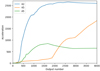 |
Fig. A.1. Evolution of the acceleration for the simulations K2, K5, and A5. |
Without the acceleration due to our handling of the CFL condition, the time interval between two outputs would have been constant, and the physical time of the solution would have been proportional to the output number. Any increase in the acceleration factor means that another batch of cells has converged. This means the time increment of the cells that are still evolving in time becomes larger, thus increasing the timescales reached.
This increase is clearly visible after the 300th output. Using the output number as a proxy for the computational cost of a simulation, this figure clearly shows that, at the end of the integration, the time boost enables us to reach timescales at least two or three orders of magnitude larger than using a standard CFL condition, without increasing the computational cost of the simulation. Analogously, without employing the time boost, we would have required two or three orders of magnitude more CPU hours to reach the same timescales. Our approach enabled us to produce simulations that would have consumed much more computing time otherwise. The reference simulation K2 consumed 725 CPU hours, but without the time boost it would have required almost two million CPU hours. This enabled us to work on simply 64 processors kindly provided by GRICAD (Grenoble Alpes Recherche - Infrastructure de Calcul Intensif et de Données).
For the evolution of the acceleration factor with the mass load, we can see in Table 1 that the simulations with κ closest to that of Blandford & Payne (1982) converge the fastest, reaching larger timescales at the end of the computation. Nevertheless, all seem to reach comparable convergence speeds: in Figure A.1 we see that the simulation K5 reaches an acceleration factor similar to that of K2 at the final output. For the evolution with the magnetic field, we can clearly see that the higher the α and thus the flatter the profile of the vertical magnetic field, the slower the simulation converges. For higher values of α, the jet is initially more collimated as Br/Bz is higher on the disk. Therefore, the field lines further on the disk have a higher impact, retarding the global convergence. That is why the simulation A5 with α = 15/16 has not yet converged. As an instability develops, some cells that were previously stable become unstable, hence the decrease in acceleration.
Appendix B: Boundary conditions
The plots represented in Figure B.1 illustrate the injection boundary conditions we have chosen for the reference simulation K2. The Bernouillli invariant E, the poloidal magnetic field BΦ, the vertical magnetic field Bz, the mass to magnetic flux ratio η = μ0ρvp/Bp, the rotation speed of the magnetic surfaces Ω⋆ = Ω − ηBΦ/(μ0ρr), the speed of sound  and vertical Alfvénic speed
  are plotted on the first cell over the injection boundary. The toroidal magnetic field goes to zero on the axis for symmetry reasons, and
  on the disk : The JED magnetic field is weakly toroidal. The launching conditions are very cold as VAz/Cs ∼ 102 on both the source and the disk.
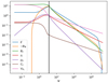 |
Fig. B.1. Conditions on the lowermost cells of the reference simulation K2. Here all parameters are traced along the first cell above the lower boundary : R = 1 and θ ∈ [0; π/2] on the source and then θ = π/2 and R ∈ [0; Rext] on the disk. Shown are the Bernouilli invariant E, the toroidal and vertical magnetic field BΦ and Bz, the mass to magnetic flux ratio η, the rotation speed of magnetic surfaces Ω*, the speed of sound Cs and the vertical Alfvénic speed VAz, over the magnetic flux Ψ. The black vertical line corresponds to the flux anchored at (R = 1,θ = π/2), at the source/disk interface. |
The reader may observe the power-law dependency with the magnetic flux on the whole disk (Ψ > 10, after the black vertical line) for all parameters but the electric current. This is directly induced by the self-similar ansatz. However, the torroidal magnetic field BΦ breaks the power-law dependency and shows a swift decrease for Ψ > 2.106. Of all eight variables, only BR and BΦ are free at the injection boundary (see Equation (8)), and need to cross a characteristic surface to be fixed. For the toroidal current, it is the Alfvénic surface. As all magnetic surfaces over Ψ ≳ 109 never cross the Alfvénic surface, the current can never be fixed. Thus, the simulation cannot ever be stationary in this region.
As the disk is a self-similar jet-emitting disk, all dimensionless parameters are assumed to be independent of the radius (Blandford & Payne 1982). All these parameters are regrouped in section 2.4.
As explained in section 2.3.2.2, we defined a spline function f(θ) equal to zero on axis (θ = 0) and one at the inner disk radius (θ = π/2) to smoothly connect the axis values with the inner disk ones: f(θ)≡(3sin2θ − 2sin3θ)3/2.
The injection speed (VR on the source, −Vθ on the disk) is fixed at κμ2 = 0.1 even when varying κ. However, even though the injection Mach number Ms = up/Cs is assumed to be the same all along the boundary, in order to account for the varying inclination of the magnetic surfaces, its value is modified with the parameter α from simulation to simulation. Its variation with α is shown in Table 1.
Appendix C: Rankine-Hugoniot jump conditions
In this section, we write the Rankine-Hugoniot jump conditions valid for standing, adiabatic recollimation shocks. Contrary to Ouyed & Pudritz (1993), we take into account the toroidal magnetic field as the shocks arise when that component is dominant. The local jump [A]=A2 − A1 between a pre-shock quantity A1 and its post-shock value A2 are expressed in the rest frame as
![$$ \begin{aligned}{[\rho u_\perp ]} = 0&\nonumber \\ {\ }[\rho u_\perp (\frac{u^2}{2} + H) + \frac{B^2}{\mu _o}u_\perp - \frac{\boldsymbol{u} \cdot \boldsymbol{B}}{\mu _o} B_\perp ] = 0&\nonumber \\ \\ {\ }[P + \rho u_\perp ^2 + \frac{B^2_\parallel - B^2_\perp }{2 \mu _o} ] =0&\nonumber \\\\ {\ } [ \rho u_\perp \boldsymbol{u}_\parallel - \frac{B_\perp }{\mu _o} \boldsymbol{B}_\parallel ] =0&\\\\ {\ } [ B_\perp ] = 0&\nonumber \\ {\ }[ B_\perp \boldsymbol{u}_\parallel - u_\perp \boldsymbol{B}_\parallel ] = 0,&\nonumber \end{aligned} $$](/articles/aa/full_html/2023/01/aa44311-22/aa44311-22-eq65.gif)
where  is the enthalpy and u⊥, B⊥ (respectively u∥, B∥ ) are the normal (respectively tangential) components to the shock surface. The shock is axisymmetric, and so the tangential component of the magnetic field B‖ = Btet + Bϕeϕ, whereas the poloidal component is Bp = Btet + B⊥e⊥, with the unit vectors (e⊥,et,eϕ) defining a local orthonormal coordinate system. As these jump conditions express the conservation of mass, angular momentum, and energy in ideal MHD, the five MHD invariants along a given magnetic surface (η, Ω*, L, E, S) are therefore also conserved (see Fig.7).
In the case of a shock, the mass flux through the surface is nonzero, which requires B⊥2 = B⊥1 ≠ 0 and leads to
where m = u⊥/VAp, ⊥ = up/VAp is the Alfvénic Mach number of the incoming (pre-shock) flow and χ = ρ2/ρ1 = u⊥1/u⊥2 is the shock compression rate. This equation shows that there are three nontrivial discontinuities with χ ≥ 1: (1) an oblique shock with m2 > χ > 1, (2) a normal shock with m2 = χ > 1 (requiring B‖1 = 0), and (3) an Alfvén shear discontinuity with m2 = χ = 1 (allowing an arbitrary jump between the two tangential field components). The oblique shock is the only case studied here.
After some algebra all post-shock quantities can be expressed as function of the pre-shock ones, in particular
where the sonic Mach number ms = u⊥/Cs and magnetic shear b2 = (B∥/B⊥)2 are computed in the pre-shock region. Of particular interest are the relative variations of the toroidal magnetic field component δBϕ = Bϕ2/Bϕ1 − 1 and the plasma angular velocity δΩ = Ω2/Ω1 − 1, as well as the total deflection angle of the poloidal magnetic surface δi = i2 − i1 where tani = Bt/B⊥, which read
These quantities are plotted in Fig. 9. The compression rate χ is the solution of the cubic polynomial equation

with
where χo = (Γ + 1)/(Γ − 1) is the maximal compression ratio for a hydrodynamic shock. Equation C.5 has one positive root only for an incoming super-FM flow, namely for n⊥ = u⊥/Vfm, ⊥ larger than unity.
We are dealing here with supersonic (ms > > 1) and super-A (m > > 1) cold jets, where the dominant magnetic field is the toroidal one (b2 ≃ (Bϕ/B⊥)2 > > 1). The FM Mach number in the normal direction therefore writes n⊥ ≃ mVAp, ⊥/VAϕ = m/b, which leads to the simplified equation for χ
This shows that whenever jets reach a very large FM Mach number n⊥, a large compression rate χ ≃ χo is possible. But this is never achieved in our case. Indeed, the poloidal FM Mach number n = up/VFM, p (> n⊥) writes
where ωA = Ω*rA/VAp, A is the fastness parameter introduced in F97 (ratio at the Alfvén point of the speed of the magnetic rotator to the poloidal Alfvén speed). For magneto-centrifugal jets like ours, with m2 > > 1, r > > rA and achieving their maximal velocity  , the FM Mach number is n2 ∼ ωA, which is larger than but of the order of unity (see also Krasnopolsky et al. 2003). As a consequence, we expect rather weak shocks as illustrated by the small values of χ achieved along the various shocks (see Fig. 9).
Figure C.1 plots the theoretical solution χth of Eq. C.5 (in yellow) computed along the main recollimation shock of our simulation K2 and compares it with the ratio χ = ρ2/ρ1 (in blue) directly measured (see Fig. 4). The correspondence is very good, with discrepancies remaining below a few percent. The two regions where larger differences are obtained correspond to the positions where the two smaller shocks (triggered at the spine-jet interface) merge with the main shock: the orange one near r ∼ 500 and the cyan one near r ∼ 900.
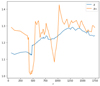 |
Fig. C.1. Distribution at tend along the main recollimation shock of the compression ratio for simulation K2. The yellow curve is the theoretical solution χth of Eq. C.5, computed using the pre-shock quantities, while the blue curve is the ratio χ = ρ2/ρ1. |
The shocks were detected by following all magnetic field lines anchored on the disk and looking for discontinuities. This is not obvious in a discrete grid. To do so, we computed the derivative of the toroidal magnetic field (δBϕ) over the curvilinear abscissa along the field line, as shocks are best seen with the electric poloidal current and explored its local extrema. We checked that a different approach, based on the calculation of the refraction angle δi of the poloidal magnetic surface, produces very similar results. This gave us the shock locations used to produce the plots in Figures 2 and 17. As PLUTO has a shock capturing scheme, each shock is resolved and has a finite width. To determine the shock width, we checked that the density was growing within the shock as expected. Then, still following the field line, we looked for the closest local minimum and maximum in density. The positions of these extrema allowed us to compute the values of the pre-shock and the post-shock quantities, respectively. These were finally used to compute the parameters leading to the Figures 9 and C.1.
All Tables
All Figures
|
Fig. 1. Sketch of our computational domain. The central object and its interaction with the innermost disk are located below the inner boundary at Rd (green region), the near-Keplerian jet-emitting disk (JED) being established from Rd to the end of the domain Rext. An axial outflow (the spine) is emitted from the central regions (in red) and the jet is emitted from the JED (in blue). The solid purple line represents a recollimation shock surface starting on the axis at a height Zc. For each point N lying on this surface, we use local poloidal unit vectors (e⊥, e∥), respectively perpendicular and parallel to the shock surface. Also, at any point M inside the domain, we either use spherical (eR,eθ,eϕ) or cylindrical (er,eϕ,ez) coordinates. |
| In the text | |
|
Fig. 2. Snapshot at tend of our Blandford & Payne simulation K2. Left: global view with field lines anchored on the disk at ro = 3; 15; 40; 80; 160; 320; 600; 1000; 1500, where the background is the logarithm of the FM mach number n. Right: close-up view of the innermost regions, where the background is the logarithm of the density. In both panels, black solid lines are the poloidal magnetic surfaces, the yellow solid lines are isocontours of the poloidal electrical current, and the red dashed (resp. dotted) line is the FM (resp. Alfvén) critical surface. |
| In the text | |
|
Fig. 3. Snapshot of our reference simulation K2 at tend. We use the same color coding as in Fig. 2, left. The black arrows show the poloidal velocity. The white lines are streamlines inside which (from left to right) 50%, 75%, and 100% of the super-FM (spine+jet) mass outflow rate is carried in. |
| In the text | |
|
Fig. 4. Close-up view of our reference simulation K2 at tend showing the shock forming region, with field lines anchored at ro = 1.2; 2; 3; 4; 5; 7; 9. The five shocks are highlighted in red, orange, cyan, blue, and purple. We use the same color coding as in the left panel of Fig. 2. |
| In the text | |
|
Fig. 5. Late evolution of several global jet quantities for the simulation K2: the radius ro, FM of the last super-FM surface, the jet mass-loss rate Ṁjet, and the two colatitudes |
| In the text | |
|
Fig. 6. Evolution of the various energy contributions along a magnetic surface of anchoring radius r0 = 100 for the simulation K2 at tend: the Bernoulli invariant E, the gravitational potential ΦG, the total specific kinetic energy u2/2, the enthalpy H, and the magnetic energy −Ω*rBΦ/η. The absicssa is the altitude Z(Ψ). |
| In the text | |
|
Fig. 7. Evolution of the MHD invariants along field lines of two different anchoring radii ro at tend for simulation K2. All invariants have been normalized to their values at ro. The absicssa is the altitude Z(Ψ). |
| In the text | |
|
Fig. 8. Evolution of several magnetic field lines during the simulation computation, for different anchoring radii R0 and for the reference simulation K2. The field lines at the first output of the simulation (initial conditions) are shown in dotted lines. The field lines at the last output of the simulation (final state) are shown as full lines. |
| In the text | |
|
Fig. 9. Distributions along the shock of several quantities for K2 at tend. Left: normal incident FM Mach number n⊥, Alfvénic Mach number m, compression rate χ, relative variations of the toroidal magnetic field δBϕ and plasma angular velocity −δΩ, and total deviation δi (in rad) of the poloidal magnetic field line for the main recollimation shock. Right: compression rates χ of all shocks appearing in Fig. 4, using the same color code. The main shock corresponds to the red curve. See Appendix C for more details on this figure. |
| In the text | |
|
Fig. 10. Radial distribution of the radial accelerations and their sum at the altitude Z = 2400 for the simulation K2 at tend. The vertical dashed line corresponds to the spine–jet interface, namely the field line anchored at ro = Rd. |
| In the text | |
|
Fig. 11. Plot of the poloidal electric circuits at tend for simulation K2. The two red curves are the critical surfaces, Alfvén (dotted) and FM (dashed). The yellow curves are the poloidal electric circuits, defined as isocontours of rBϕ, where the arrow indicate the direction of the poloidal current density Jp. Four circuits are highlighted in particular: (1) the envelope of the inner accelerating current in white (rBϕ = −2.06), (2) the outermost circuit still fully enclosed within the domain in blue (Bϕ = −2.005), (3) a circuit closed outside the domain in orange (rBϕ = −1.80), and (4) a post-shock accelerating circuit in purple (also with rBϕ = −2.06). |
| In the text | |
|
Fig. 12. Altitude Z of the different shocks (measured at the axis) as a function of time (in Td units) for simulation K2. The vertical lines correspond to the six times ti used in Fig. 13: t1 = 551, t2 = 2.08 × 10³, t3 = 8.51 × 10³, t4 = 1.99 × 10⁴, t5 = 1.05 × 10⁵, and t6 = 1.58 × 10⁵. The last vertical line is tend = 6.51 × 10⁵. |
| In the text | |
|
Fig. 13. Snapshots of our reference simulation K2 at different times (given in Td units). From top to bottom, left to right: t1 = 551, t2 = 2.08 × 10³, t3 = 8.51 × 10³, t4 = 1.99 × 10⁴, t5 = 1.05 × 10⁵, and t6 = 1.58 × 10⁵. The background color is the logarithm of the density, black lines are the magnetic surfaces, red lines the Alfvén (dotted) and FM (dashed) surfaces, and yellow curves are isocontours of the poloidal electric current. |
| In the text | |
|
Fig. 14. Time evolution of the cylindrical radius r measured at Z = 3500 of the magnetic surface anchored at ro = 3 (blue curve) and the electric current I = rBϕ (red) flowing within that surface for simulation K2. The two vertical dashed lines correspond to t5 = 1.05 × 10⁵ and t6 = 1.58 × 10⁵. |
| In the text | |
|
Fig. 15. Jet parameter space λ(κ) at the final stage of our simulations K1–K5 with α = 3/4. Each simulation is obtained for a unique mass loading κ and gives rise to a distribution of the magnetic lever arm λ with the radius: green, red, and blue dots correspond to anchoring radii ro = 5, 50, and 500, respectively. The solid curves are obtained for constant values (indicated in the panel) of the initial magnetic field inclination |
| In the text | |
|
Fig. 16. Influence of the mass-loading parameter κ on the final stage of jets obtained with α = 3/4. The color background is the logarithm of the FM Mach number n, black solid lines are field lines, yellow lines are isocontours of the electric current rBϕ and the red dashed (resp. dotted) curve is the FM (resp. Alfvén) critical surface. The left panels show the whole domain and the right panels a close-up view around the shock-formation regions. In the left panel, the field lines anchoring radii are ro = 3; 15; 40; 80; 160; 320; 600; 1000; 1500. In the right panel, the field lines anchoring radii are ro = 1.2; 2; 3; 4; 5; 7; 9; 11; 13; 15. |
| In the text | |
|
Fig. 17. Influence of κ (orange lines) and α (blue lines) on the altitude of the main recollimation shock. This is done by measuring two altitudes for each shock: its height at the axis (Zshock, solid lines) and the altitude of its outer edge (Ztip, dashed lines). The scale for κ is indicated below, while the scale for α is above. |
| In the text | |
|
Fig. 18. Influence of the magnetic field distribution α on the final stage of jets obtained with κ = 0.1. We use the same notations, colors, and field lines anchoring radii as in Fig. 13. |
| In the text | |
|
Fig. 19. Snapshot at tend of our SP simulation with a rotating spine, α = 3/4 and κ = 0.1. We use the same color coding as in Fig. 2. The magnetic field lines (black solid lines) are anchored at the same disk radii. |
| In the text | |
|
Fig. A.1. Evolution of the acceleration for the simulations K2, K5, and A5. |
| In the text | |
|
Fig. B.1. Conditions on the lowermost cells of the reference simulation K2. Here all parameters are traced along the first cell above the lower boundary : R = 1 and θ ∈ [0; π/2] on the source and then θ = π/2 and R ∈ [0; Rext] on the disk. Shown are the Bernouilli invariant E, the toroidal and vertical magnetic field BΦ and Bz, the mass to magnetic flux ratio η, the rotation speed of magnetic surfaces Ω*, the speed of sound Cs and the vertical Alfvénic speed VAz, over the magnetic flux Ψ. The black vertical line corresponds to the flux anchored at (R = 1,θ = π/2), at the source/disk interface. |
| In the text | |
|
Fig. C.1. Distribution at tend along the main recollimation shock of the compression ratio for simulation K2. The yellow curve is the theoretical solution χth of Eq. C.5, computed using the pre-shock quantities, while the blue curve is the ratio χ = ρ2/ρ1. |
| In the text | |
Current usage metrics show cumulative count of Article Views (full-text article views including HTML views, PDF and ePub downloads, according to the available data) and Abstracts Views on Vision4Press platform.
Data correspond to usage on the plateform after 2015. The current usage metrics is available 48-96 hours after online publication and is updated daily on week days.
Initial download of the metrics may take a while.