Accretion rates of 42 nova-like stars with IUE and Gaia data

Roberto Gilmozzi; Pierluigi Selvelli

doi:10.1051/0004-6361/202244014

Home

All issues

Volume 681 (January 2024)

A&A, 681 (2024) A83

Full HTML

Open Access

Issue		A&A Volume 681, January 2024


Article Number		A83
Number of page(s)		21
Section		Stellar structure and evolution
DOI		https://doi.org/10.1051/0004-6361/202244014
Published online		22 January 2024

A&A 681, A83 (2024)

Accretion rates of 42 nova-like stars with IUE and Gaia data

Roberto Gilmozzi¹ and Pierluigi Selvelli²

¹ European Southern Observatory, Karl Schwarzschild-Str. 2, 85748 Garching, Germany
e-mail: rgilmozz@eso.org
² INAF – Osservatorio Astronomico di Trieste, Via Tiepolo 11, 34143 Trieste, Italy
e-mail: selvelli@oats.inaf.it

Received: 13 May 2022
Accepted: 28 July 2023

Abstract

We analyzed more than 700 ultraviolet spectra of 45 nova-like stars (NLs) observed with the International Ultraviolet Explorer (IUE) satellite, obtaining reliable data for 42 of them. Combining these with the distances from the Gaia Early Data Release 3 (EDR3) and with results from the literature, for each object we determined the reddening E_B − V, the disk spectral energy distribution (SED), the reference (i.e., inclination-corrected) absolute magnitude and disk luminosity (M_V^ref, L_disk^ref), and the mass accretion rate (Ṁ), all with propagated errors. The de-reddened UV continuum of NLs in a high state is well approximated by a power-law distribution with index α in the range −2.4 ≤ α ≤ −0.2. The agreement between the power-law extrapolation to the V band and the observed V magnitude is outstanding and implies that for NLs in a high state, the disk continuum dominates not only in the UV but also in the optical, with other possible contributions (white dwarf, M dwarf, and hot spot) being minor. We note that the accretion rate correlates with the period, power-law index, and M_V^ref, making them convenient proxies for Ṁ. The strongest correlation (p_H₀ < 10⁻⁶) is log Ṁ = −0.57 ± 0.06 M_V^ref−5.98 ± 0.29. Nine of the 42 NLs fall within the period gap but all have Ṁ very similar to that of the objects above the gap, contrary to theory expectations but in agreement with other observational work, and indicating that − at least for NLs − the theoretical assumptions of the standard model of the evolution of CVs need substantial revision. Medians and weighted means of log Ṁ (≈ −8.5) are very similar among NL classes, and also to those of old novae, dispelling the prejudice that stars belonging to the SW Sex class of NLs have “exceptionally high” Ṁ compared to other NLs (and old novae). In fact, it is one of the most interesting results of this study that NLs and old novae are indistinguishable in terms of Ṁ and its correlation with M_V^ref. Two NLs (V1315 Aql and BZ Cam) have shells around them, a likely fingerprint of a past nova eruption, but the suggested association with “guest stars” of ancient Chinese chronicles is questionable.

Key words: accretion, accretion disks / novae / cataclysmic variables / ultraviolet: stars / stars: distances

© The Authors 2024

Open Access article, published by EDP Sciences, under the terms of the Creative Commons Attribution License (https://creativecommons.org/licenses/by/4.0), which permits unrestricted use, distribution, and reproduction in any medium, provided the original work is properly cited.

This article is published in open access under the Subscribe to Open model. Subscribe to A&A to support open access publication.

1. Introduction

Nova-like stars (NLs) are a class of non-magnetic cataclysmic variables (CVs) characterized by a generally high luminosity and, unlike dwarf novae (DNe), by the absence of disk outbursts. The high and mostly stable luminosity is indicative of a high accretion rate (Ṁ) that keeps the optically thick disk in a stable state (Osaki 1974; Meyer & Meyer-Hofmeister 1984; Smak 1984, 2002; Patterson 1984; Shafter 1992; Ballouz & Sion 2009; Townsley & Gänsicke 2009; Hoard et al. 2014; Dubus et al. 2018). However, in some members of the class, the high state is interrupted by occasional and unpredictable low states that can last for weeks to years (see Sect. 3.2). The classification of NLs is not straightforward since it depends on the adopted photometric and/or spectroscopic criteria. Hereafter, following Sion & Godon (2022), the NLs in a steady high state are called UX UMa stars, while the systems with occasional low states are called VY Scl. On the basis of spectroscopic criteria, some members of these two classes can also be classified as SW Sex stars (see Sect. 3).

Cataclysmic variables are short-period semidetached binary systems in which a white dwarf (WD) primary accretes material from a Roche lobe filling secondary, generally a late-type near-main-sequence star. For an introductory review of the current knowledge of CVs, readers can refer to Szkody & Gaensicke (2012). CVs are the end point of binary star evolution and ideal laboratories for the study of the physics of mass transfer and mass accretion processes. The orbital period (P_orb) of CVs is short (about 1 to 10 h) and the main sequence star generally fills its Roche lobe and transfers mass onto the white dwarf through the L₁ Lagrangian point, in a semidetached configuration. Because the orbital angular momentum of the accreting matter is high, matter is not transferred directly onto the WD and, unless the WD is strongly magnetic, an accretion disk is formed around the WD where gravitational potential energy is released through viscous heating and is balanced by radiative cooling (for comprehensive considerations on CVs, see Warner 1995; Frank et al. 2002; Smith 2007; Knigge 2011; Postnov & Yungelson 2014).

The standard model of CV evolution is that the P_orb of these systems would decrease on timescales of 10⁸ − 10⁹ years due to mass transfer and angular momentum losses (Knigge 2011; Hoard et al. 2014). Therefore, the mass accretion rate (Ṁ) is a fundamental parameter for our understanding of the evolution of CVs. As mass starts being transferred between the stars in a semidetached system, both the components’ masses and the orbital separation change. In the case of conservative mass transfer (where the total mass and angular momentum of the binary remain fixed), if a low-mass star accretes onto a higher mass star, as in the case of CVs, the star separation and P_orb increases and consequently the donor star loses contact with its Roche lobe and mass transfer subsequently stops. Thus the very action of mass transfer in such systems would result in the cessation of further mass transfer (Shafter et al. 1986). Mass transfer continues if the binary loses angular momentum and, as a consequence, the orbit shrinks and contact ultimately resumes.

The standard paradigm of CV evolution assumes that orbital angular momentum losses (AMLs) are driven by mechanisms such as gravitational radiation (Faulkner 1971; Paczynski & Sienkiewicz 1981) dominating in systems with P_orb < 3 h (see also Spruit & Ritter 1983; Howell et al. 2001; Knigge 2006; Knigge et al. 2011) and magnetic braking (MB) by a magnetic stellar wind (MSW) from the secondary (Eggleton et al. 1976; Rappaport et al. 1983; Verbunt & Zwaan 1981; Gänsicke 2004; Davis et al. 2008), dominating in systems with P_orb > 3 h. The knowledge of AML rates is crucial for understanding CV evolution since evolution is driven by AMLs from the binary orbit. AML rates are generally estimated by determining the mass accretion rate.

The MB scenario requires the presence in the secondary star of a magnetic field with open lines in order to drain angular momentum from the system. The open magnetic field lines of the secondary drive the stellar wind to large radii while forcing the wind to corotate with the star up to the Alfven radius where the wind becomes free and is lost to the star. This large amount of angular momentum lost from the secondary is eventually redistributed to the system as a whole because, in short, P_orb binary systems’ tidal forces between the stars tend both to circularize the orbits and to synchronize the rotation and orbital periods. Thus, the angular momentum lost by the tidally locked secondary and carried away in its magnetic wind is ultimately extracted from the system as a whole, causing the binary system to shrink and the P_orb to decrease. This maintains the contact of the secondary with its Roche lobe and guarantees continuity of the mass transfer. It should be pointed out, however, that tidal friction is by no means well understood (Eggleton 2011).

The need for a process such as MB for the long-term evolution of CVs arises from the fact that the observed mass transfer rates can exceed those driven by gravitational radiation (GR) alone by more than one order of magnitude. The rates of mass transfer via MB are typically 10⁻⁹ − 10⁻⁸ M_⊙ yr⁻¹, which is much higher than the rate of mass transfer due to GR (about 10⁻¹⁰ M_⊙ yr⁻¹) in short-period CVs (Howell et al. 2001).

The MB mechanism is believed to dominate for systems in which the secondary star has a radiative core and a convective envelope since the magnetic dynamo action is thought to occur at the interface between the two (Spruit & Ritter 1983). This corresponds to a secondary mass M₂ larger than about 0.3 M_⊙, or equivalently P_orb ≥ 3 h in the Roche configuration (Frank et al. 2002). At P_orb ≤ 3 h, the secondary star is predicted to become fully convective and magnetic braking is thought to be no longer effective. The disrupted magnetic braking (DMB) scenario explains the famous (or infamous) period gap, that is, the apparent abrupt decline of the Ṁ in CV systems with P_orb less than about 3 h where, allegedly, only the less effective gravitational radiation is at work for AMLs. In the standard model (Knigge 2011), it is generally accepted that MB stops abruptly when the secondary becomes fully convective at around M₂ ∼ 0.3 M_⊙. As a consequence of inefficient MB, the system loses contact and the CVs enter the period gap (2.15–3.18 h, Knigge 2006) as a detached system: this cuts off the mass transfer and the system becomes much fainter. The result is the scarcity of observed CVs inside the period gap, whose presence is of crucial importance for understanding the evolution of CVs (Willems et al. 2005; Knigge et al. 2011). Mass transfer restarts when further loss of angular momentum via gravitational radiation has reduced the orbital separation and the P_orb has decreased to around 2 h. (Rappaport et al. 1983); for specific details, readers can refer to Knigge et al. (2011).

2. Comments on the AML-DMB mechanism

It should be noted that the AML-DMB mechanism sketched above has been the subject of criticism for various reasons (for details see Knigge et al. 2011):

To obtain their magnetic braking law prescription (or conjecture, Hameury 1994) Verbunt & Zwaan (1981) extrapolated over several orders of magnitudes the work of Skumanich (1972) on the spin-slowing down rate of isolated G-type stars by a MSW (i.e., from the slow rotation rates of single field star to the expected high rotation rates of the secondaries of close binaries).

The DMB scenario depends crucially on the assumption that MB suddenly stops when the secondary becomes fully convective. However, there are several examples of low mass presumably fully convective single stars that are magnetically active (Smith 2007). Also, no discontinuous decline in magnetic activity for fully convective stars is evident (Davis et al. 2008; Jones et al. 1996). In fact, as pointed out by Eggleton (2011), the activity persists to much lower masses with many low-mass M dwarfs showing magnetic activity (see also Donati 2006). In this case no gap would be formed, in contrast with the commonly accepted interpretation of the period gap. Thus far there has been no observational evidence for an abrupt change in spin-down rate due to MB between late-type field stars that are fully convective and those that have a radiative core (Andronov et al. 2003); see also Kafka & Honeycutt (2006) for the magnetic properties of low mass stars. Very recently El-Badry et al. (2022) found that the intrinsic period distribution of low-mass (0.1 ≲ M₁/M_⊙ ≤ 0.9) binaries is basically flat (dN/dP_orb ∝ P_orb) from P_orb = 10^d down to the contact limit. They also found no significant difference between the period distributions of binaries containing fully and partially convective stars. Since the period distribution is a sensitive probe of MB, they concluded that MB in CVs is much weaker than assumed in the standard evolutionary model.

The MB mechanism leads (practically independent of the value of P_orb at the time of becoming a CV) to the prediction of a tight relationship between Ṁ and P_orb (Warner 2000). AMLs depend essentially only on the binary period and as a consequence similar Ṁ are expected in different systems at the same P_orb (King 1988; Kolb & Ritter 1992). Only this would guarantee the coherence of the phenomenon (Ritter 2012). Instead a large spread (by more than one order of magnitude) in the mass transfer rates at a given P_orb is observed (Patterson 1984; Warner 1995; Kolb 2001; Spruit & Taam 2001; Ritter 2012; Woudt et al. 2012; Dubus et al. 2018). Note that the recent work of Pala et al. (2022) seems to indicate a lower spread only for systems below the period gap, most of them dwarf novae.

The evolution toward shorter P_orb has been challenged by Borges & Baptista (2005) who pointed out that well studied CVs do not show evidence of period decrease but just cyclical period changes, probably associated to solar-type magnetic activity cycles in the secondary star. See also the study by Dai et al. (2010) who reported a definite increase in the P_orb of the SW Sex star V348 Pup that they considered as part of a long term modulation.

Shafter (1992) declared that the period gap is only clearly defined for DNe. Baptista et al. (1993) suggested that there was no period gap for novae. Kolb (1996) also pointed out that the observed distribution of periods in novae shows no signature of a gap. Verbunt (1997) reanalyzed the period distribution of CVs and came to the conclusion that for nova-like systems the period gap is not significant. Hellier & Naylor (1998) also indicated that the period period gap is not significant in NLs.

It should be noted that all CVs, irrespective of their subtypes, are included in the period distribution showing the period gap (including the magnetic systems which instead do not show a gap), with mostly NLs at longer P_orb and mostly DNe at shorter ones. This raises the possibility that the gap may be an artifact due to treating different classes as if they had the same properties.

3. The NLs subclasses

NLs come in a number of subtypes depending on their photometric properties and/or spectroscopic behavior (see Introduction). For simplicity from here on we use the term class for UX UMa, VY Scl, SW Sex and non-SW Sex stars, and NL for the whole sample.

3.1. UX UMa

UX UMa stars are characterized by a hot and luminous disk indicative of high Ṁ. Unlike in DNe, the high Ṁ, above the critical value of ∼1.5 10⁻⁹ M_⊙ yr⁻¹, keeps the optically thick disk in a stable state (Osaki 1974; Meyer & Meyer-Hofmeister 1984; Smak 1984; Patterson 1984; Shafter 1992). As a consequence the accretion disk is the dominant luminosity source from the far UV to the optical range to the IR (Hoard et al. 2014). Therefore, observations of UX UMa stars, particularly in the UV, provide an excellent opportunity to investigate the physical characteristics of a steady state accretion disk. UX UMa stars have periods in the range 2.5 ≤ P_orb ≤ 8 h.

3.2. VY Scl

The members of the VY Scl class are affected by the anti-dwarf-nova syndrome: they spend most of their time varying little about a mean magnitude but occasionally show rapid drops in brightness by 1.5–7 mag, with most objects in the range 3–5 mag (La Dous 1994; Warner 1995; Dhillon 1996). These episodes can last for weeks to years (Hameury & Lasota 2002; Rodríguez-Gil et al. 2012). In these low states the disk is not the dominant source of luminosity, and contribution by other components, especially the hot WD, is likely. Most VY Scl systems have P_orb of 3–4 h, just above the period gap.

3.3. SW Sex

Several UX UMa and VY Scl systems can be also classified as belonging to the SW Sex class. The SW Sex class was proposed by Thorstensen et al. (1991; but see also Honeycutt et al. 1986; Dhillon 1996) for a few highly inclined (eclipsing) systems and is characterized by a number of spectral features that set them apart from other NLs, such as (1) single-peaked emission lines even in high inclination systems, (2) transient absorption features in the emission lines, (3) distorted radial velocity curves, and (4) high excitation level in the spectra, including very strong He II 4686 emission, see also Hoard & Szkody (1997), Hoard et al. (2003), Rodríguez-Gil et al. (2007a), Schmidtobreick (2017). Several new objects with SW Sex characteristics were discovered since the original work, including in low inclination systems. According to Rodríguez-Gil et al. (2007b) SW Sex stars represent nearly 50% of the CVs with period between 3 and 4.5 h. Nearly 40% of the SW Sex stars are not eclipsing binaries. See also the D.W. Hoard’s Big list of SW Sextantis stars¹.

It should be noted that the class of SW Sex is not universally accepted: neither the FUSE survey of CVs by Froning et al. (2012; where most of the SW Sex stars are classified as NL-UX UMa) nor the CVCAT by Downes et al. (2006) adopt it. Also, Hameury & Lasota (2002) do not include SW Sex stars in their study of CVs.

Dhillon (1996) pointed out that the SW classification is debatable, since SW Sex stars can only be recognized by their spectroscopic properties, whereas other subclasses of CVs are classified on the basis of their photometric properties. Therefore the SW Sex classification overlaps with other classifications. Following Hoard et al. (2010) one could summarize this as “SW Sex stars are NLs CVs, although not all NLs are SW Sex stars”.

3.4. non SW Sex

The plots and histograms show also the non SW Sex objects in order to assess if there is any information to be gained by their data.

4. The purpose of this work

NLs are found above and below the upper boundary of the period gap and therefore their study is fundamental for our understanding of CV evolution in this critical period range. In particular, with the set of homogeneous data from IUE and Gaia for 42 NLs, we plan to derive accurate Ṁ values in order to:

1. Verify the reality for NLs of one of the basic paradigms of CVs evolution that associates higher accretion rates to systems with longer P_orb (Howell et al. 2001). Early studies of the observed Ṁ in CVs (see Patterson 1984) indicated a strong dependence of Ṁ on the P_orb. Patterson (2011) substantially confirmed the correlation between M_V (taken as a proxy for Ṁ) and P_orb, although with a weaker dependence. It should be noted, however, that these results derived essentially from optical observations of DNe in outburst and have been, somewhat arbitrarily, extrapolated to CVs in general.

2. Test with a statistically significant and homogeneous sample of NLs whether different NLs at the same P_orb have different Ṁ (as reported in previous studies lacking accurate distances, e.g., Patterson 1984; Warner 1995; Kolb 2001; Spruit & Taam 2001; Woudt et al. 2012). If confirmed, this is a major problem in the theory of binary evolution.

3. Verify the existence itself and the amount of the expected drop in the Ṁ for the NLs with P_orb inside the period gap.

4. Check the claims of exceptionally high Ṁ in SW Sex systems compared to other CVs (Rodríguez-Gil et al. 2007a,b; Schmidtobreick et al. 2012; Schmidtobreick & Tappert 2015).

5. Compare and contrast the Ṁ of the various classes of NLs including that of the old novae. The SW Sex stars represent a significant fraction among NLs and understanding their relation to the other members of NLs would represent a major improvement of our understanding of CV evolution (Gänsicke 2004).

6. Compare the Ṁ values derived by us using IUE data and Gaia distances with those obtained using similar IUE data with accretion disk models.

5. The key role of IUE and Gaia in determining Ṁ

The spectroscopic wavelength range of the International Ultraviolet Explorer (IUE) satellite (1150–3200 Å, hereafter UV) is of the utmost importance for the study of CVs since most of their accretion luminosity is emitted at these wavelengths (Wade 1988). Patterson (1984) showed that Ṁ (the non plus ultra of binary evolution according to Patterson 2011) can be directly estimated using the optical luminosity of the accretion disk. However, reliable statements about Ṁ can be made only for objects that have well determined distance and reddening as well as observations covering the satellite UV range where most of the accretion luminosity is emitted.

The combination of IUE’s UV spectra with the latest precise parallaxes from the Gaia satellite EDR3 release (Gaia Collaboration 2021) has provided critical input for a direct estimate of the luminosity and mass accretion rate for the NLs of our sample with good quality UV spectra.

6. The input data

6.1. The IUE spectra

The IUE databank contains more than 700 low resolution UV spectra obtained with the short wavelength prime (SWP) and the long wavelength prime and redundant (LWP, LWR) cameras for 45 NLs present in the catalogs of Ritter & Kolb (2011) and Downes et al. (2006), the lists of Warner (1995), Puebla et al. (2007) and Ballouz & Sion (2009), and the comprehensive study by La Dous (1991).

The spectra used in this paper were retrieved from the IUE Newly Extracted Spectra (INES) final archive. For a detailed description of the IUE-INES system see Rodríguez-Pascual et al. (1999) and González-Riestra et al. (2001).

Of the retrieved spectra we selected the 614 taken with the large aperture (to avoid throughput losses). Three objects (V1082 Sgr, V1776 Cyg and VZ Scl) have only low quality spectra and were disregarded.

For the remaining 42 objects, all 614 spectra were examined and both of those with a very low signal-to-noise ratio (S/N < 5) and those with a low and intermediate IUE flux (indicative of a low state in the VY phenomenon) were disregarded. We also disregarded spectra with bad agreement between the SWP and the LWP/LWR spectral regions. These selections left 289 high quality spectra available.

Since the study of the small short-time variations of the continuum in individual objects is beyond the scope of the present study (most spectra have exposure times comparable to or longer than the P_orb), all high state individual spectra with similar flux level were co-added, averaged and merged into a single λλ 1170–3200 Å representative spectrum, with the exclusion of UU Aqr and V380 Oph for which only SWP spectra were secured. The improved S/N in the average spectra has allowed a more accurate determination of continuum slope and reddening correction.

Table 1 gives the list of objects, the number of SW and LW spectra for each and the range of dates in which they were taken.

Table 1.

IUE spectra: numbers per camera and totals (extract).

6.2. The basic parameters and their uncertainties

Table 2 lists the basic data for the 42 NLs in Col. 1, that is the UX UMa or VY Scl classification (Col. 2), the SW Sex classification (Yes/No/Probable, Col. 3), the P_orb (Col. 4), the system inclination i (Col. 5), and the distance d (Col. 6).

Table 2.

Basic parameters.

The SW classification follows Hoard et al. (2003) “Big List of SW stars”. To avoid introducing a “probable SW” class of only 5 elements we have merged these objects with the certain ones for the analysis and plots.

The P_orb’s (Col. 4) are mostly from Ritter & Kolb (2011), with uncertainties that are negligible for the rationale of this study and are not included in Table 2. We note that for HQ Mon Bruch & Diaz (2017) give also P_orb = 5.16 h. We chose the value of Ritter & Kolb (2011) for homogeneity with the other data and because of the long familiarity with the source.

For the remaining basic parameters we assumed as nominal value the average of the various values found in the literature. We adopted as error bar the semi-difference of their range; therefore errors for these quantities are not statistical but rather indicate the likely ranges for the parameters values. We are aware that in doing so we probably overestimated the errors (see discussion in Selvelli & Gilmozzi 2019, Appendix A).

The case of V426 Oph is an intriguing one: it is listed as a NL in the General Catalog of Variable Stars (GCVS) and in Patterson (1984), and as a NL-UX UMa in Ritter (1984), but is listed as a Z Cam in Warner (1995), Downes et al. (2001), and Dubus et al. (2018). Hellier et al. (1990) discussed the possibility of it being an intermediate polar but concluded it was not. Ramsay et al. (2008) pointed out that there is a great deal of uncertainty as to the subtype of V426 Oph. We have taken a pragmatic approach after noticing that in all the plots used to derive correlations V426 Oph is indistinguishable from all the other objects so we used it in our fits. Figures 3, 6 and 8 show V426 Oph with a larger symbol to help the comparison.

6.3. The distance from Gaia-EDR3

The Gaia Early Data Release 3 (Gaia Collaboration 2021) provides precise positions, proper motions, and parallaxes (ϖ) for an unprecedented number of objects (almost 1.5 billion). Data for all NLs of our sample are contained in this release. Since the ϖ uncertainties, with the exception of KR Aur, are below 2% we have followed the naive approach of calculating the distances as 1/ϖ. Column 6 of Table 2 gives distances with errors. Note that for consistency the distance of KR Aur is also from 1/ϖ. We have compared it with the EDR3 one using the method by Bailer-Jones (2015), Luri et al. (2018) and Bailer-Jones et al. (2018). The EDR3 distance is within 3% of the previous one (459 ± 53 vs. 445 ± 47), with the luminosity L_ref within 6% and log Ṁ changing from −8.86 to −8.83, so we consider the 1/ϖ value quite acceptable.

6.4. The period distribution

Histograms of the period distributions for the UX/VY and SW/nSW classes are shown in Fig. 1 (top). Although overlapping, a difference in the distribution between classes is clearly evident, with the SW and VY classes having tighter distributions peaking at shorter periods (around 3.9 h), while the UX class is spread more evenly (average ≈5.0 h, see Table 3, top). It is possible that the period segregation of SW and VY stars is a defining characteristic of these classes (see Conclusions). Nine NLs (V592 Cas, V795 Her, MV Lyr, AH Men, KQ Mon, V442 Oph, LQ Peg, V348 Pup, and LX Ser fall into the period gap (see Sect. 8.2 for a discussion of the similarity of their Ṁ to that of NLs above the gap).

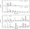Fig. 1.

Histograms of the periods (above) and inclinations (below) of the NLs in this paper, according to their class(es). The period gap (Knigge 2006) is indicated in the upper panel. Note that in the two panels of each figure the NLs are the same, but divided according to their class. To avoid confusion the histogram bins for each pair of classes have been plotted on either side of the central values, with sizes that avoided contact between adjacent bins.

Table 3.

Class averages of distributions of periods and inclinations.

6.5. The system inclination

The inclination is critical to estimate many parameters (e.g., $M_{V}^{ref}$ $M_V^{{\rm ref}}$ , $L_{disk}^{ref}$ $L^{\mathrm{ref}}_{\mathrm{disk}}$ and Ṁ, see Sects. 7.4–7.7). In particular, since the observed luminosity comes from the accretion disk, a correction for the angle of view of the disk is necessary in order to compare NLs among themselves. In Table 2, Col. 5, the adopted values for the inclination are mostly from the compilation by Ritter & Kolb (2011), supplemented by additional information from the literature on individual objects (see note to Table 2). Inclination averages per class are in Table 3. For a few objects (WX Ari, QU Car, RZ Cru, CM Del, V442 Oph, and V3885 Sgr) there are contradictory estimates of i in the literature. For these also we have used the average values and their (larger) uncertainties (see Appendix A.1 for details).

We note that with the exclusion of UX UMa all systems with i > 64 degrees are SW Sex stars. It is surprising that there are almost no members of the nSW class in eclipsing systems (see discussion in Sect. 8.5).

Figure 1 (bottom) shows the histograms of the cos i distributions of NLs according to their classes. The distributions of UX, VY and SW are rather homogeneous while that of nSW is biased toward lower inclinations, as indicated above, raising the possibility that there are nSW objects that appear as belonging to a different class if seen at high inclination.

6.6. The observed optical magnitude

In Sect. 7.3 the optical magnitude (m_v) will be compared to the magnitude obtained from the extrapolation of the UV power law to the V range. For this comparison we inspected the data from the AAVSO, Ritter & Kolb (2011) and Downes et al. (2006) to derive the m_v in a high state for all objects and especially for the VY Scl class. This for homogeneity with the IUE spectra that were chosen from high state only. With few exceptions (see below) the three sets of (m_v) data are in good agreement. This approach allowed for an estimate of the uncertainties in m_v from the visual inspection of the AAVSO data, since the Ritter & Kolb (2011) and Downes et al. (2006) catalogs do not include errors. The final values in Col. 4 of Table 4 are mostly from the AAVSO with few exceptions (see below). The Ritter & Kolb (2011) and Downes et al. (2006) point values generally fall within the given errors range.

Table 4.

Main results of this study.

It is desirable to have m_v data as close as possible in time to those of the IUE observations. We did so when AAVSO data were available. In the other cases we used the available AAVSO data even if not contiguous to the IUE observations since the Ritter & Kolb (2011) and Downes et al. (2006), usually closer to the IUE observations, also agreed with the AAVSO values. Moreover these objects were in stable high states throughout the available data.

Three objects (TT Ari, KR Aur, and DW UMa) have brighter m_v (Ritter & Kolb 2011 and Downes et al. 2006) values compared to those from the AAVSO. We used the AAVSO values for these objects:

TT Ari. Ritter & Kolb (2011) and Downes et al. (2006) give m_v = 9.5; we determined 10.6 ± 0.5, a value in agreement with Jameson et al. (1982) 10.2 − 11.8 (note that these values were closer to the times of the UV observations).

KR Aur. Ritter & Kolb (2011) and Downes et al. (2006) give 11.3, we determined 13.3 ± 0.6, in agreement with Hutchings et al. (1983) who indicated m_v ∼ 13 − 14. Also these values were closer to the IUE observations.

DW UMa. Ritter & Kolb (2011) and Downes et al. (2006) give 14.9, we choose 14.2 ± 0.3 supported by many AAVSO observations and by Honeycutt et al. (1993) who found 14.2, and by Boyd (2009) who found 14.2 as the typical magnitude.

Two objects (HL Aqr, V348 Pup) have no AAVSO data:

HL Aqr. Verbunt (1997), Ritter & Kolb (2011), Downes et al. (2006), Puebla et al. (2007) give 13.4–13.6. Recent DR3 Gaia data give 13.5 in filter BP (centered at lambda ∼5300 Å). The value in Table 4, 13.3 ± 0.2, is in good agreement with those above.

V348 Pup. Rolfe et al. (2000), Ritter & Kolb (2011), Downes et al. (2006), Puebla et al. (2007), all give 15.5, Gaia DR3 gives 15.82 B, 15.7 G. The value in Table 4, 15.6 ± 0.2, is in good agreement with those above.

In any case it is worth pointing out that this is a statistical study of NLs properties, and small variations in a few data points do not affect the final results (as proven post facto by the excellent correlation coefficients presented in this paper).

6.7. Remarks on propagation of errors and correlations

An important aspect of this study is the determination of the uncertainties of the basic physical quantities and their propagation to the final, most significant parameters, that is the disk accretion luminosity and Ṁ. This was achieved using the Python environment that provides specific modules and packages² that allow calculation of the propagation of errors.

Some figures show linear fits between variables (or their log). These are based on Deming (1943) regressions (an early instance of maximum likelihood estimation) because they account for errors in both x and y and therefore are, in our opinion, more realistic than standard $1 / σ_{y}^{2}$ $1/\sigma_{\it y}^2$ weighted fits. Since Deming fits do not provide error estimates for the coefficients we have determined them using the Jackknife (resampling) method originally introduced by Quenouille (1949) and Tukey (1958), in the modern version from Numerical Recipes (2007, Cambridge University Press).

We used the Pearson’s coefficient r_P to test for possible correlations between quantities. The requirements for the two-tailed null hypothesis probability (p_H₀) were set to be rather strict: < 10⁻² for believable correlations and < 10⁻³ for strong ones. Both r_P and p_H₀ are shown in the figures containing fits, but giving the most significant power of 10 for p_H₀.

7. Results

This section reports the results of this study (see Table 4).

7.1. The reddening correction and the UV continuum SED

The UV range is most sensitive to the effects of reddening, since it is characterized by the almost ubiquitous presence of a broad interstellar absorption feature centered near λ 2175 Å. A simple and common method for estimating the reddening is that of removing the 2175 Å feature in the observed spectrum.

We used the method we followed in Selvelli & Gilmozzi (2019), which is based on the Cardelli et al. (1989) correction. Varying the correction in steps of 0.01 mag we determined the E_B − V as the intermediate value between those where a weak absorption bump or a weak emission bump were still appreciable in the spectra. The extremes have been taken as the uncertainty of the determination. A power law (PL) fit to the de-reddened spectra proved to be an excellent representation of the SED.

We tested the results using a less interactive method: in the assumption that the intrinsic SED is indeed a power law we fit both reddening and PL simultaneously to the original spectra (see examples in Fig. 2). The spectra were σ-clipped to minimize the contribution of the lines, and 3-pixel smoothed prior to the fit. The fitting code produced coefficients and their errors.

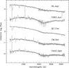Fig. 2.

Examples of simultaneous fits of power law and reddening to IUE spectra.

The two methods yielded excellent agreement in most cases. For these, the values in Table 4 of the PL coefficients and their errors are those from the simultaneous fit. The values of E_B − V and related errors are from the interactive method as it is independent of spectral shape assumptions.

There were a few cases (identified in the table by an asterisk) where the shape of the spectrum was not a clear reddened PL. For these the PL parameters are from the fit to the de-reddened spectra. It is interesting, however, that the extrapolation of these PLs to the V band (see Sect. 7.3) provides magnitudes very similar to those observed, offering a sort of a posteriori support to the plausibility of the PL and reddening parameters.

Two objects, UU Aqr and V380 Oph, have far-UV SWP spectra only and therefore it is somewhat more difficult to fit PL and E_B − V to them since the most important feature, the 2175 Å bump, is not in the spectrum. We have however applied the method of fitting PL and E_B − V simultaneously to these SWP spectra and obtained estimates of the parameters. The fact that the extrapolation of the PL to the optical provides also in this case magnitudes similar to those observed gives us confidence in the results obtained.

We tested the results for UU Aqr and V380 Oph against the IPAC reddening maps (2011) and the Stilism (Capitanio et al. 2017) database that includes distance dependent reddening estimates. IPAC gives E_B − V = 0.12 ± 0.02 and E_B − V = 0.15 ± 0.00 respectively while Stilism gives 0.06±0.02 and 0.18±0.07 respectively. The values determined by us (Table 4) are E_B − V = 0.14 ± 0.04 and E_B − V = 0.12 ± 0.04 respectively, in excellent agreement with the IPAC results and slightly off with respect to the Stilism database.

The E_B − V = 0 result for V825 Her, LQ Peg and V348 Pup may appear odd, particularly in the case of V348 Pup which has a Galactic latitude of −11 deg. IPAC gives E_B − V = 0.02 for V825 Her, E_B − V = 0.08 for LQ Peg and E_B − V = 0.20 for V348 Pup, while Stilism gives E_B − V’s of 0.02 (at 500 pc), 0.045 (at 600 pc) and 0.11 ± 0.01 respectively.

Given that the IPAC values are upper limits for our objects (IPAC gives the total galactic reddening in a given direction), and that the Stilism values are averages over large areas (typically ≳ arcmin²), we do not find the reddening of these three NLs suspicious.

7.2. The expected correlation between α_PL and cosi

Accretion disk models (Wade 1988) show that the spectrum of an accretion disk has a slope that critically depends, for a given Ṁ and WD mass, on the inclination angle.

Figure 3 (top) shows the PL index α against the cosine of the system inclination angle for all NLs in the sample. The immediate impression from the figure is that there is a large spread of α values for any given inclination. There are however four correlations: the whole, UX and SW at p_H₀ < 10⁻⁴ and the VY at p_H₀ < 10⁻². The nSW class shows no correlation, possibly because of its skewed inclinations distribution (all but one object have cos i > 0.49, see Fig. 1 and Sect. 8.5). The graphs, fit lines and relevant statistical parameters for the strongest correlations are shown in Fig. 3.

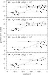Fig. 3.

Power-law index vs. the cosine of the inclination angle. The panels display the four correlations at p_H₀ < 10⁻², i.e., from the top the whole sample, the UX, VY, and SW classes, each with their respective correlation parameters and fits. The nSW class shows no correlation. V426 Oph is highlighted with a square box (see last paragraph of Sect. 6.2 for details).

It is our opinion that this result confirms the presence of the expected correlation between the power law index and cos (i), although with large scatter: the functional relation

$\begin{matrix} α = - 3.44 \pm 0.66 \cdot cos i + 0.60 \pm 0.42 \end{matrix}$ $\begin{aligned} \alpha = -3.44\pm 0.66 \cdot \cos i + 0.60\pm 0.42 \end{aligned}$ (1)

has a large rms (0.80) that is clearly dominated by the uncertainties in the inclination angle. It would be difficult to consider this a way to determine one of the parameters if the other is known, not least because a fit with very different relative errors in the variables is very challenging; for more details, readers can refer to Ihn (2016), Asuero et al. (2006), and Draper (1991), for example.

The fact that such a high correlation coefficient is present (−0.59 at p_H₀ < 10⁻⁴) shows, however, that a correlation does exist. This result is at variance with the statement by Verbunt (1987) that the slope shows no clear correlation with inclination (although, like Verbunt (1987), we find no correlation between slope and period). It should also be noted that Godon et al. (2017) from a study based on IUE spectra, reported the absence of a definite correlation between i and the far UV continuum slope α.

Two objects, V363 Aur and UX UMa, have well established inclinations larger than 70 degrees, although both exhibit a rather steep continuum slope. V363 Aur has i = 71 ± 7, see Rutten et al. (1992), Ritter & Kolb (2011), La Dous (1991), Warner (1995), Thoroughgood et al. (2004), Bisol et al. (2012), Puebla et al. (2007). Our determination of the UV continuum slope (α = −1.93) is the same as Bisol et al. (2012; −1.93) and Godon et al. (2017; −1.9). UX UMa has i = 70 ± 5 (Petterson 1980, Warner 1995, Ritter & Kolb 2011, Wade 1988, La Dous 1991, Ramsay et al. 2017, Bruch 2021, Neustroev et al. 2011, Knigge et al. 1998, Linnell et al. 2008, Noebauer et al. 2010, Baptista et al. 1995, Puebla et al. 2007). We found α = −1.83, while Godon et al. (2017) give α = −2.0.

There are five other objects (QU Car, CM Del, RZ Gru, V442 Oph and V3885 Sgr) with an alleged (but partially uncertain) inclination close to 60 degrees (see Appendix A.1 for details) that also exhibit a steep continuum slope in the range −2.3 < α < −1.7, see Table 4 for the individual values. This is at odds with the behavior expected from common wisdom and accretion disk modeling that indicate that in high Ṁ, disk dominated objects such as NLs in high states, a steep continuum slope is generally associated to a disk seen in a low inclination system, see La Dous (1989, 1991) and Wade & Hubeny (1998).

Some possible scenarios, for example a tilted accretion disk as suggested in the case of PX And and V795 Her by Thomas et al. (2010), an extreme flare up of the disk edge, or the prograde apsidal precession of an eccentric disk, as suggested by Patterson et al. (2002) would allow us to see a larger fraction of the disk than expected from the inclination angle and may help explain the phenomenon. Unfortunately there are not enough data in our set to explore these options in any rigorous way.

7.3. The optical magnitude and the extrapolation of the UV power law continuum to the V band

The PL fit to the UV SED can be extrapolated to the V range and the derived magnitude (V_PL), after reddening (i.e., V_PL + A_V), can be compared to the observed m_v (to determine what if any is the disk contribution to the optical range.). Column 5 of Table 4 gives the V_PL + A_V values while Fig. 4 shows their comparison with the AAVSO magnitudes.

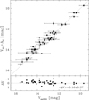Fig. 4.

Extrapolation of the UV power law to the V band (V_PL) after applying the reddening correction versus the AAVSO V observations around the dates the IUE spectra were taken. The tight agreement shows that most of the flux in the V band comes from the disk.

The agreement is outstanding (weighted average difference 0.16 ± 0.37 mag, see also Sect. 8.7 for further comments), and this implies that for NLs in a high state the disk continuum dominates in both the UV and optical ranges, with other possible contributions (WD, M dwarf, and hot spot) being minor.

7.4. Inclination correction to the observed magnitude and luminosity

Since most of the flux comes from the disk, a correction for the inclination angle needs to be applied to compare the various NLs: two identical objects at i = 0 and i = 90 will have very different observed properties (Warner 1986, 1987). Following the procedure described in Sect. 8 of Selvelli & Gilmozzi (2019) we have calculated the reference (i.e., inclination independent) values of disk magnitudes, fluxes and luminosities using

$\begin{matrix} M v_{ref} = M v_{obs} - Δ M v (i) \end{matrix}$ $\begin{aligned} M\mathrm{v}_{\rm ref}=M\mathrm{v}_{obs}-\Delta M\mathrm{v} (i) \end{aligned}$ (2)

$\begin{matrix} L_{disk}^{ref} = 3.116 \cdot 10^{4} \times d^{2} \int_{1100}^{6000} (F_{λ} d_{λ} \times f_{λ}^{- 1} (i)) \end{matrix}$ $\begin{aligned} L_{\rm disk}^\mathrm{ref} = 3.116 \cdot 10^4 \times d^2 \int _{1100}^{6000} (F_{\lambda } d_{\lambda } \times f_{\lambda }^{-1} (i) ) \end{aligned}$ (3)

where the inclination dependent correction terms were computed for both the Webbink et al. (1987; WLTO) and the Paczynski & Schwarzenberg-Czerny (1980; hereafter PSC) prescriptions:

$\begin{matrix} f_{λ} (i) = 2 cos (i) \end{matrix}$ $\begin{aligned} f_{\lambda } (i)=2 \, \cos (i) \end{aligned}$ (4)

$\begin{matrix} Δ M_{v} (i) = - 2.5 log (2 cos (i)) \end{matrix}$ $\begin{aligned} \Delta M_{\rm v} (i)=-2.5 \log \, (2 \, \cos (i)) \end{aligned}$ (5)

for the WLTO correction, and

$\begin{matrix} f_{λ} (i) = [1 - u_{λ} + u_{λ} cos (i)] cos (i) / (0.5 - u_{λ} / 6) \end{matrix}$ $\begin{aligned} f_{\lambda } (i)=[1-u_ {\lambda }+u_ {\lambda } \cos (i)] \cos (i)/ (0.5-u_{\lambda }/6) \end{aligned}$ (6)

where u(λ) = 0.85 − 4.1667 × 10⁻⁵ λ, and

$\begin{matrix} Δ M_{v} (i) = - 2.5 log (f_{v} (i)) \end{matrix}$ $\begin{aligned} \Delta M_{\rm v} (i)=-2.5 \log \, (f_{\rm v} (i)) \end{aligned}$ (7)

for the PSC correction (please note that the PSC formula in our old novae paper, Selvelli & Gilmozzi 2019, had a missing cos i). For the V band (u_v = 6) Eq. (6) simplifies to

$\begin{matrix} f_{v} (i) = [1 + 1.5 cos (i)] cos (i), \end{matrix}$ $\begin{aligned} f_{\rm v} (i)= [1+1.5\, \cos (i)]\, \cos (i), \end{aligned}$ (8)

that is the Warner (1987) formula that of course was used to compute ΔM_v(i) in the PSC case.

7.5. The reference absolute magnitude versus the inclination

Columns 6, 7 of Table 4 give $M_{V}^{ref}$ $M_V^{{\rm ref}}$ with errors for the two inclination corrections (with the subscripts W and P). A comparison of the two corrections shows that they are in fair agreement (they differ by 0.10 ± 0.27 mag), although the PSC one tends to overcorrect $M_{V}^{ref}$ $M_V^{{\rm ref}}$ at high i, introducing a larger scatter. The WLTO correction, instead, shows less spread and a more uniform distribution of objects with high and low i.

There is no correlation between $M_{V}^{ref}$ $M^{\mathrm{ref}}_{\mathrm{V}}$ and i for the whole or any class (a sort of a posteriori validation of the inclination correction). In fact, a spread of up to 2 mag is present at any given i. Figure 5 shows the histograms of $M_{V}^{ref}$ $M_V^{{\rm ref}}$ (top) and of log Ṁ (bottom) for the various classes. Table 5 gives their means and medians.

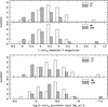Fig. 5.

Histograms of the reference absolute V magnitude (top) and of the accretion rate (bottom) for the various classes.

Table 5.

Weighted means (WM) and medians (Med) of $M_{V}^{ref}$ $M_V^{{\rm ref}}$ (top) and log Ṁ (bottom).

We note that the nine objects inside the gap (2.15–3.18 h, Knigge 2006) have $M_{V}^{ref}$ $M_V^{{\rm ref}}$ similar to that of the objects above the gap, see Fig. 4 and also the comments in Sect. 8.2.

7.6. The reference absolute disk luminosity

Given the results in Sect. 7.3 one can estimate the total disk flux, or at least provide a reliable (lower) limit for the sum of the UV and optical contributions by integrating the PL from 1100 to 6000 Å. In turn, the observed total disk luminosity can be directly derived using the accurate Gaia distances of Table 2.

We neglected the possible (and in any case small) IR contribution to the disk luminosity (Hoard et al. 2002) by truncating the integral of the PL at 6000 Å. This choice is supported by the fact that we observed in T Pyx (Gilmozzi & Selvelli 2007) that the magnitudes beyond the V band are progressively fainter than the extrapolation of the PL to those wavelengths, indicating that beyond the V band the disk becomes optically thin – or has a physical edge.

We also disregarded the far-UV contribution at λ < 1100 Å because far UV observations by FUSE (see Froning et al. 2004, 2012) show that NLs show a steep decrease of the UV continuum below that wavelength; for more details, readers can refer to the HUT observations of IX Vel by Long et al. (1994), for example. Accretion disk models (Wade & Hubeny 1998) confirm this and show a sharp decline below λ 1100 Å.

Table 4 Cols. 8 and 9 show $L_{ref}^{disk}$ $L_{\mathrm{ref}}^{\mathrm{disk}}$ for both i corrections. It is reassuring that the two corrections give results that differ at most by a factor two, with an average $L_{W}^{disk} / L_{P}^{disk}$ $L^{\mathrm{disk}}_{W}/L^{\mathrm{disk}}_{P}$ of 0.92 ± 0.28.

Since the relative corrections show the same difference as in the case of $M_{V}^{ref}$ $M_V^{{\rm ref}}$ , from here on we use values based on the WLTO prescription for $M_{V}^{ref}$ $M_V^{{\rm ref}}$ and $L_{ref}^{disk}$ $L_{\mathrm{ref}}^{\mathrm{disk}}$ (and derived quantities such as Ṁ), but report also the data using the PSC correction in the tables. Consequently the correction subscripts are omitted in the rest of the paper.

The intrinsically most luminous disk is QU Car with $L_{disk}^{ref} = 42.2 \pm 5.5 L_{⊙}$ $L^{\mathrm{ref}}_{\mathrm{disk}} = 42.2 \pm 5.5\,L_\odot$ .

7.7. The observed mass accretion rate

Following Selvelli & Gilmozzi (2019), Ṁ has been derived from $L_{disk}^{ref}$ $L_{\mathrm{disk}}^{\mathrm{ref}}$ as:

$\begin{matrix} \dot{M} = 5.23 \cdot 10^{- 10} ϕ L_{disk}^{ref} / L ⊙, \end{matrix}$ $\begin{aligned} \dot{M}=5.23 \cdot 10^{-10}\, \phi \,\, L^\mathrm{ref}_{\rm disk}/L\odot ,\end{aligned}$ (9)

where ϕ = 125 R_WD/M_WD, with radius and mass in solar units, is the inverse efficiency in converting Ṁ into luminosity.

We used ϕ = 1.765, corresponding to M_WD = 0.76 ± 0.10 M_⊙, the weighted means of the 29 NLs in our sample that have WD masses in the literature. The data were mostly from Ritter & Kolb (2011), supplemented by additional information from Araujo-Betancor et al. (2003), Ballouz & Sion (2009), Baptista et al. (1995), Bisol et al. (2012), Bruch (2021), Dhillon et al. (1997), Dubus et al. (2018), Hessman (1988), Hoard & Szkody (1997) Martínez-Pais et al. (2000) Mizusawa et al. (2010), North et al. (2002), Poole et al. (2003), Puebla et al. (2007), Ramsay et al. (2017), Smak (2019), Thoroughgood et al. (2004), Vande Putte et al. (2003), Young & Schneider (1981).

The value we found (0.76 ± 0.10M_⊙) is in good agreement with the average CV WD mass of $0 . 81_{- 0.20}^{+ 0.16} M_{⊙}$ $0.81^{+0.16}_{-0.20} \ M_\odot$ very recently found by Pala et al. (2022) from a sample of 89 CVs. Knigge et al. (2011) found M_WD = 0.77 M_⊙ above and M_WD = 0.73 below the period gap. Instead, Pala et al. (2022) found no evidence of any correlation of the WD mass with P_orb.

Columns 10 and 11 of Table 4 give log Ṁ and errors for the two inclination corrections. They differ by 0.05 ± 0.15. Table 5 gives weighted means and medians of the various classes for the WLTO correction, showing that SW and nSW classes have log Ṁ very similar to that of the whole sample (≈ − 8.6), while UX and VY objects show a higher and a lower value (by 0.2) respectively. All accretion rates are however well within the error bars of each of the classes.

QU Car is the most luminous NL in our sample and likely the most luminous NL (Drew et al 2003). QU Car was proposed as a candidate V Sge star (Hoard et al. 2014; Kafka et al. 2008). These objects have an evolved secondary star that allows very high mass transfer rates near the Eddington limit (∼ 10⁻⁶ M_⊙ yr⁻¹) that would lead to stable nuclear burning on the surface of the WD (see Kafka et al. 2008 and Steiner & Diaz 1998). However, the observed Ṁ in QU Car (∼ 4 × 10⁻⁸ M_⊙ yr⁻¹) is much lower than the Eddington limit and not compatible with the classification of QU Car as a V Sge star (see also Oliveira et al. 2014).

An extreme case of discrepant Ṁ estimates in the literature is that of RW Tri, an eclipsing object with a well-defined inclination of 76 ± 7 (cf. Ritter & Kolb 2011: 70 ± 3, La Dous 1991: 82, Warner 1995: 75, Mizusawa et al. 2010: 71 ± 3, Hoard et al. 2014: 75, Puebla et al. 2007: 60−80). Previous Ṁ determinations (Wade 1988, Cordova & Mason 1985, Frank & King 1981, Horne & Stiening 1985, Mizusawa et al. 2010) span 3 orders of magnitude: 10^−7.8 to 10^−10.8 M_⊙ yr⁻¹ (see also Cordova & Howarth 1987). The value derived in this paper is 10^{−8.92 ± 0.24} M_⊙ yr⁻¹.

7.8. The possible contribution by the WD

In recent studies, the modeling of the UV SED includes a possible WD contribution to the observed UV flux, for example in Godon et al. (2017), Sion et al. (2009), and Mizusawa et al. (2010).

Simple calculations seem to exclude this at least for our NLs in a high state. Their average luminosity is ∼3 L_⊙, while even in the case of the presence of a very hot WD with T ∼ 45 000 K (extrapolating to the whole NLs class the T reported by Pala et al. 2022 for three VY Scl systems), most of the WD luminosity (∼0.37L_⊙) would be emitted below 1100 A with a minor contribution to the IUE and optical ranges.

As mentioned in the Introduction, a WD contribution to the UV and V flux is expected only for VY Scl (anti-DN) systems in low state (when the disk becomes optically thin and the WD is expected to show high temperatures due to heating by the disk during the decline phase). Interestingly, Pala et al. (2017) reported very high WD temperatures for 3 such systems, based on a study by Townsley & Gänsicke (2009). The low states of TT Ari, MV Lyr and DW UMa showed WD temperatures around 39 000, 47 000 and 50 000 K respectively.

These three objects are in our sample and simple calculations show that the V flux from the disk is brighter than that in low state by 6.7, 5.3 and 4.7 mag, respectively. A direct comparison between the derived V magnitude from the WD alone and that of the observed AAVSO magnitudes shows that for TT Ari and MV Lyr the difference is of ∼6 mag while for DW UMa is ≳4 mag. These differences correspond exactly to the observed deep luminosity drops of these objects during low states and indicate the hot WD as the main source of the V light in these minima (the possible contribution by the red companion being lower by about 2 mag).

The presence of a possible boundary layer at T ⪆ 200 000 K (necessary to doubly ionize He to produce the observed 1640 Å line) would not be detectable in IUE’s UV range: its peak would be at much shorter wavelengths and its area very small, making its Rayleigh-Jeans tail contribution to the rest of the disk negligible.

7.9. Comments on Ṁ from standard accretion disk models

In the pre-Gaia era, several UV-based studies of NLs provided estimates of Ṁ (see Puebla et al. 2007; Hamilton et al. 2007; Ballouz & Sion 2009; Mizusawa et al. 2010; Bisol et al. 2012; Wolfe et al. 2013) based on the model spectra for steady state accretion disks by Wade & Hubeny (1998).

However, Orosz & Wade (2003) pointed out that, given the inability to model steady disks in well studied systems, one cannot rely on model fitting to give the correct Ṁ for systems of unknown distances, adding that UV observations of nova-like variables are very difficult to fit using steady disk models constructed from LTE stellar atmospheres.

Cannizzo (1998), from a study of DNs in outburst, also concluded that one cannot rely on model fitting to give the correct luminosities or mass accretion rates (within an order of magnitude). Similar conclusions have been reached by Knigge et al. (1998) and by Froning et al. (2003). See also Godon et al. (2017) for recent discussions on the modified spectral modeling and the use of the TLUSTY and SYNSPEC suite of codes.

Puebla et al. (2007) in a study of 23 NLs systems, most of them included in our larger sample, noted that models are too blue compared with the observed spectra, and also pointed out that there is a strong degeneracy among the parameters within disk models. Their analysis with fixed distance gave an average log Ṁ ∼ −8.03 (compared to −8.61 ± 0.38 in the present study). The distance was also assumed as a free parameter to allow the matching of the observed flux level, but this attempt resulted in inconsistent and too low values for the distance.

In general, a comparison between the distances from synthetic spectral fitting and those from Gaia EDR3 (in parenthesis in the list below) shows that the best fitting model distances are systematically lower than those of Gaia EDR3 (by factors of up to six). For example: AH Men: 116 (499) pc; LQ Peg: 350 (1280) pc; TT Ari: 65 (249) pc (Ballouz & Sion 2009); V795 Her: 159 (572) pc; V425 Cas: 278 (928) pc; HL Aqr: 213 (580) pc (Mizusawa et al. 2010); KQ Mon: 155 (628) pc (Wolfe et al. 2013); V363 Aur: 134 (841) pc; RZ Gru: 116 (563) pc; AC Cnc: 105 (639) pc (Bisol et al. 2012).

It is therefore understandable that many of the values for Ṁ derived in the present study (Table 4) do not agree with those derived in the studies based on synthetic spectral fitting models. As an exception see Sect. 8.8 for comments on the Ṁ values of SW and nSW derived by Ballouz & Sion (2009).

7.10. A note on Ṁ from other methods

In this study we have derived the mass accretion rate Ṁ of NLs starting from the observed UV accretion disk luminosity and accurate distance determination from Gaia.

It is worth mentioning that Patterson (1984) in his fundamental study derived Ṁ in CVs (DNe at max, old novae, NLs) using just the observed optical magnitude m_v and rather approximates estimates of the distances. Nevertheless his statistical study clearly confirmed the correlation between m_v (taken as a proxy for Ṁ) and P_orb associating higher Ṁ to systems with longer P_orb, which constitutes the basic paradigm for the interpretation of CVs evolution.

In recent papers, the technique of using the observed luminosity of the accretion disk to estimate Ṁ has been criticized for being sensitive to a short observational baseline.

Townsley & Gänsicke (2009) suggested that the WD temperature is a more reliable tracer of the secular transfer rate. Regrettably, this technique is almost useless for NLs. For the VY Scl systems it requires far UV observations during their almost unpredictable low states, while for the UX UMa it is unfeasible owing to their permanent high luminosity that prevents a direct detection of the WD. In short: in UX UMa stars the WD temperature is not an observable. Pala et al. (2022) have recently estimated the secular Ṁ for three members of the VY Scl class but for DW UMa, the only object in common with us, they found a quite high log Ṁ = −7.64 (our value is ∼ –8.40) and the object was considered as an outlier.

The technique of the WD temperature of Townsley & Gänsicke (2009) to determine the secular Ṁ has been criticized by Knigge et al. (2011) who, alternatively, consider the measure of the radius of the secondary star as the most reliable tracer of the long term mass transfer rate since the secondary radius is a measure of its state of thermal equilibrium. However, this technique is also of limited application because it is restricted to eclipsing NLs only: recent studies of M-dwarf stars (Parsons et al. 2018; Morrell & Naylor 2019; Morales et al. 2022) have shown that there are uncertainties in the mass-radius relationship in low mass stars, with growing evidence that M-dwarf stars suffer radius inflation when compared with theoretical models.

Therefore, whether the WD temperature or the radius of the secondary are more reliable tracers of the secular mass accretion rate seems still matter of debate.

It should be pointed out that Willems et al. (2007) determined the secular mean mass transfer rate in DNe as the product of the mass accretion rate during outburst times the duty cycle. For DNe they assumed 0.1 as duty cycle, while for nova-like CVs they assumed 1.0 since the objects are persistently bright.

It turns out that NLs are steady accretors, with Ṁ larger than the critical Ṁ rate for disk instability that separates NLs from DNe. This guarantees a persistently high mass transfer rate, which is confirmed by the steadiness, during many decades, of the observed M_v in this class. This steadiness is also supported by our IUE observations: in all cases where spectra taken at different epochs and with time separation of years were available they presented a near constancy in the UV flux level.

In any case, the average Ṁ values for the various classes can be considered as representative of their respective long term accretion rates (see Table 5 and Fig. 10).

8. Discussion

The data of Table 4 can be used to check the validity of some generally accepted paradigms and to test whether the classes of NLs systems show peculiar characteristics.

In this section we discuss this and in particular we test the data for presence or absence of correlation between Ṁ and other system parameters.

8.1. Ṁ and the orbital period

A correlation between the observed Ṁ and P_orb is generally assumed in the basic paradigm of CVs (Patterson 1984). Figure 6 shows Ṁ vs. P_orb for the various classes in the sample. The x-axis is shown in log to dilute the crowding of data at short periods.

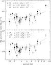Fig. 6.

Mass accretion rate vs. period. Relevant correlation parameters are given for all classes. Linear fit lines to the UX and nSW classes (dashed) as well as the whole sample (dotted) are plotted. They appear curved because the x-axis is rendered in log to avoid crowding of data at short periods. V426 Oph is highlighted with a square box (see last paragraph of Sect. 6.2 for details).

Although Ṁ shows a spread of up to one order of magnitude for any P_orb, the correlation parameters show that correlations exist for the whole and for the UX and nSW classes. The linear fits vs. P_orb for these two classes are plotted in the respective panels as dashed lines while the fit to all NLs (dotted line) is plotted in both panels. The curved shape is due to the logarithmic x-axis.

The functional relation for all NLs (at p_H₀ < 10⁻³) is:

$\begin{matrix} log \dot{M} = 0.098 \pm 0.046 P_{orb} - 9.08 \pm 0.20, rms = 0.30 \end{matrix}$ $\begin{aligned} \log \dot{M} = 0.098\pm 0.046 \,\, P_{\rm orb} - 9.08\pm 0.20, \ \ \ \mathrm{rms=0.30} \end{aligned}$ (10)

showing that P_orb is a proxy for Ṁ (to within a factor of two). A weak correlation between Ṁ and P_orb was determined by Puebla et al. (2007) with a trend not very different from ours, although with somewhat higher accretion rates (not surprising since the distances they used were derived from disk models, and these were often quite different from the Gaia ones, see Sect. 7.9).

It is intriguing that no such correlation was found in our earlier work (Selvelli & Gilmozzi 2019) on classical novae (CNe). This may be an unlikely consequence of the smaller sample (18 objects), but could also indicate that CNe represent indeed a special class of CVs, not representative of the intrinsic properties of CVs, confirming previous considerations by Truran & Livio (1986), Ritter (1990), Politano et al. (1990), Ritter et al. (1991) and Livio (1992a,b), whose theoretical works seem to suggest that the mean WD mass in old novae could be much higher (between 1.04 and 1.24 M_⊙) than in other CVs.

8.2. Ṁ and the period gap

It is worth emphasizing that for the nine objects with P_orb inside the gap (2.15 to 3.18 h, Knigge 2006) mentioned in Sect. 6.4 there is no evidence of the expected drop in the mass accretion rate, which is in fact indistinguishable from that above the gap (if not even slightly higher). Figure 7 shows a comparison of the Ṁ versus P_orb distribution of the NLs in this paper with the results of a study by Dubus et al. (2018) on the disk instability model in a sample of ∼130 CVs. The combined data show that most of the objects within the gap have Ṁ comparable to that of the objects above it.

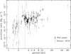Fig. 7.

Comparison of accretion rates vs. period in this paper (black dots) with the data by Dubus et al. (2018; gray dots).

This result represents a major challenge to the commonly accepted model of CV evolution (see Spruit & Ritter 1983; Knigge et al. 2011; Zorotovic & Schreiber 2020) according to which near the upper edge of the period gap the secondary star becomes fully convective and the abrupt shut off of the magnetic dynamo results in a disruption of the magnetic braking efficiency, in a loss of contact with the Roche lobe and in a sharp drop or cessation of the mass transfer rate, with expected Ṁ ∼ 5 10⁻¹¹ M_⊙ yr⁻¹ (see also Ritter 2012, and Knigge et al. 2011, the latter summarizing the situation as “There is no mass transfer in the gap“).

In an alternative view, Garraffo et al. (2016, 2018) following an idea by Taam & Spruit (1989) and observational evidence against the decline of magnetic activity in late M dwarfs, have suggested a model in which the period gap is a consequence of an increase in the magnetic complexity of the secondary star near the long-period edge of the gap. The more complex field shuts down the wind and drastically reduces the magnetic braking, resulting in a sharp decline in AML with a corresponding drop in the accretion rate.

We reiterate that the Ṁ data of Dubus et al. (2018) as well as those of the NLs in this paper show neither a sharp nor a gradual decline inside the gap.

Our results also show that the five UX UMa stars and the four VY Scl stars inside the gap have Ṁ values close to the average of their classes (see Table 5). The percentage of SW Sex systems inside the gap (seven out of nine) is higher than the average.

It is worth mentioning that Verbunt (1997) suggested that the period gap is not significant for NLs if the VY Scl systems are classified not as NLs but as DNe. Hellier & Naylor (1998) argued against this classification and concluded that NLs show a cutoff at about 3 h.

It is not clear to us whether these high Ṁ systems entered the gap as a result of evolution or were formed in the gap with mass transfer turn-on inside the gap. D’Antona et al. (1989) modeled a few cases of formation inside the gap but, regrettably, they do not seem relevant to our case. Their Model 2 (M₂ = 0.20 M_⊙) corresponds to P_orb below the gap, while in Model 3 (M₂ = 0.35 M_⊙) magnetic braking similar to Verbunt & Zwaan (1981) is included as a sink of angular momentum (although the star is considered fully convective) and, in the standard evolution model, this is not applicable for objects inside the gap.

It is worth noting that Politano (1990) reported that CVs may form in the period gap although at a rate about an order of magnitude lower than the peak rates of formation at other periods.

In any case, the observed high Ṁ, inside the gap, similar or higher than that observed above it, requires that magnetic braking (or some other unknown mechanism) is still very active for all nine objects inside the gap. Apparently, all these systems are in a semidetached configuration, contrary to the commonly accepted paradigm that CVs evolve as detached systems across the period gap, (Davis et al. 2008; Zorotovic et al. 2016). This represents a major challenge to the common model of CV’s evolution, according to which CVs evolve through the period gap as detached systems with cessation of the mass transfer.

8.3. On period gaps and Gaia gaps

We cannot help speculating that the period gap could arise from a lack of M dwarfs near M₂ ≈ 0.35 M_⊙ as recently observed in Gaia surveys (Jao et al. 2018; Feiden et al. 2021), see also Perryman & Zioutas (2022). They have pointed out that there is a pronounced discontinuity in number density of the coolest red dwarfs. Accordingly, the gap would arise because of the very different internal structure of stars on either side of it. The convective motion in the fully convective core of low mass stars (below 0.35 M_⊙) would help mix the intermediate nuclear fusion products. The mixing occurs over a narrow range of masses, with an associated dip in the luminosity function which would be responsible for the observed gap. It is our opinion that the coincidence of this gap with the period gap in CVs is very interesting and deserves a detailed investigation.

8.4. Ṁ and the inclination

There is no correlation between the two. Since Ṁ is computed from parameters corrected for inclination this is not surprising, but the absence of residual correlation could be seen here as well as a post facto validation of the i-correction and Ṁ estimates.

8.5. Ṁ and the power law index α

There is a strong correlation between the two (at p_H₀ < 10⁻⁴) that is quite interesting because the index α is a fit to the de-reddened IUE spectra, that is without correction for inclination. Therefore the estimate from the equation below can be used also for systems whose inclination is unknown:

$\begin{matrix} log \dot{M} = - 0.36 \pm 0.07 \cdot α - 9.14 \pm 0.11, rms = 0.28 \end{matrix}$ $\begin{aligned} \log \dot{M} = -0.36\pm 0.07 \cdot \alpha - 9.14\pm 0.11,\ \ \ \mathrm{rms=0.28} \end{aligned}$ (11)

indicating that α can be used as a proxy for Ṁ within better than a factor of two.

Figure 8 shows the fit to the whole sample. The two panels show the class subdivisions: UX and VY (top) and SW and nSW (bottom). The relevant correlation parameters are reported in each panel and show that all classes correlate with α at least at p_H₀ < 10⁻². The nSW have a steeper slope (≈ − 0.8) than the whole or the other classes (≈ − 0.3). This may due to the combination of their segregation in α (≤ − 0.9) and the consequent higher relative weight of QU Car (the rightmost object in the plot with the highest α and Ṁ), although a fit without QU Car still gives a steeper slope (≈ − 0.6). Given that nSW are also segregated in inclination with all but one having cos i ≥ 0.5 (Fig. 1) this may indicate again that the “missing” nSW objects at high inclination have characteristics that make them appear as members of another class.

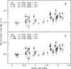Fig. 8.

Mass accretion rate vs. power law index for UX and VY (top) and for SW and nSW (bottom). Correlation parameters are given for each class, the fit (same in both panels) is to the whole sample. V426 Oph, at α ∼ −2, is highlighted with a lozenge (see last paragraph of Sect. 6.2 for details).

It is intriguing that the range − 1.05 > α > −1.65 is populated only by four stars (all both VY and nSW and with rather low Ṁ), although they are too few to derive any inference (see also comments in Sect. 8.7 about some VYs possibly not being at maximum).

8.6. Ṁ and the reference absolute magnitude $M_{V}^{ref}$ $\mathit{M\,}_{\mathsf{V}}^{{\mathsf{ref}}}$

It is clear from the results in Tables 3 and 5 that for the NLs in our sample Ṁ is high enough to mask both the WD and the companion contributions. To quantitatively test this, also in view of the match between observed V_AAVSO magnitude and the extrapolation of the PL to the V band (Sect. 7.3), we compared the Ṁ values derived in Sect. 7.8 with the $M_{V}^{ref}$ $M_{V}^{\mathrm{ref}}$ values derived in Sect. 7.5.

Figure 9 shows a clear correlation between log Ṁ and $M_{V}^{ref}$ $M_{\mathrm{V}}^{\mathrm{ref}}$ that confirms that the optical magnitude comes mainly from the accretion disk. A linear fit to the data gives

$\begin{matrix} log \dot{M} = - 0.58 \pm 0.07 M_{V}^{ref} - 5.95 \pm 0.33, rms = 0.27 \end{matrix}$ $\begin{aligned} \log \dot{M} = -0.58\pm 0.07\,\, M_{\rm V}^\mathrm{ref} -5.95\pm 0.33, \ \ \ \ \ \mathrm{rms} = 0.27 \end{aligned}$ (12)

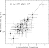Fig. 9.

Mass accretion rate vs. reference absolute V magnitude, showing a strong correlation between the two. In fact, at p_H₀ < 10⁻⁶ this is the strongest correlation in this paper.

indicating that the i-corrected absolute visual magnitude of NLs in a high state is also a proxy for Ṁ, to better than a factor of 2. In fact, at p_H₀ < 10⁻⁶ it is the best correlation among the data of this study (the UX, SW and nSW each show correlation at p_H₀ < 10⁻⁴, while VY show one at p_H₀ < 10⁻²).

Note that an equally strong correlation exists also for the absolute magnitude not corrected for the inclination:

$\begin{matrix} log \dot{M} = - 0.47 \pm 0.06 M_{AAVSO} - 6.45 \pm 0.26, rms = 0.27 \end{matrix}$ $\begin{aligned} \log \dot{M} = -0.47\pm 0.06\,\, M_{\rm AAVSO} -6.45\pm 0.26, \ \ \ \ \ \mathrm{rms} = 0.27 \end{aligned}$ (13)

providing yet another proxy for Ṁ to within better than a factor of two that is applicable in general and especially for cases in which the inclination is unknown.

Puebla et al. (2007) also found a correlation between Ṁ and M_V with a trend similar to ours, although the caveat about distances and higher accretion rates mentioned above (Sect. 8.1) applies here as well.

8.7. The Ṁ of UX and VY systems

About 57% of NLs in our sample are affected by the VY syndrome that is almost equally distributed, by number, between SW and nSW systems, see Cols. 2 and 3 of Table 2. VY objects have typically a lower log Ṁ (≈ − 8.8) than the steady NL accretors UX stars (∼ − 8.4).

It may have been tempting to interpret this as a defining characteristic of the class. However, as indicated by the difference of 0.22 mag in the average V magnitude of UX and VY, this is probably simply due to the fact that a number of VYs were not at maximum when observed with IUE (see Sect. 7.3).

Note that without the VY stars the difference between AAVSO magnitudes and the PL extrapolation decreases to 0.06 ± 0.35 strengthening the arguments above.

8.8. The Ṁ of SW and nSW systems

It is sometimes mentioned as an accepted fact that the Ṁ in SW stars is “extremely high” or “most extreme” (Rodríguez-Gil et al. 2007a,b; Schmidtobreick et al. 2012; Schmidtobreick & Tappert 2015). Actually these statements appear based on thin evidence: Rodríguez-Gil et al. (2007a,b) extrapolated the indication that DW UMa is very bright to the whole SW class, defining it as “well above their CVs cousins”, while Groot et al. (2004, but see also Neustroev et al. 2011), suggested that the classification of a NL as UX UMa/RW Tri or SW depends mostly on its Ṁ.

In the bottom panels of both Figs. 6 and 8 the SW and nSW stars are plotted with different symbols, and it is evident that they are essentially indistinguishable as far as Ṁ is concerned. Their weighted averages and medians are listed in Table 5 and plotted in Fig. 10, confirming this. It is intriguing that SW and nSW stars have nearly identical average log Ṁ ∼ −8.6 in spite of their different P_orb and i distributions (Fig. 1).

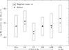Fig. 10.

Comparison of medians and weighted means of the mass accretion rates of NLs and their classes (calculated for the average 0.76 M_⊙ WD mass) with that of classical novae (calculated for 1 M_⊙ WD mass, see text for details).

We conclude that our results refute the statements reported above about higher Ṁ being a defining characteristic in the classification of SW stars.

Note that Ballouz & Sion (2009), in an IUE based study of fifteen NL variables, most of them also in our sample, derived Ṁ from synthetic spectral fitting models and found no significant differences between the Ṁ of the SW and nSW systems, in agreement with our results based on a larger sample. Also, their average log Ṁ values for SW and nSW (respectively −8.40 and −8.52) are close to ours and within our error bars.

This is a matter of some surprise since their best fitting model distances (their Table 3) are systematically lower than those of Gaia EDR3 by factors of up to 4, see Sect. 7.9.

9. Comparing the Ṁ of NLs and old novae

The nature of NLs and its relationship to CNe is not well established. A comparison between the Ṁ of old novae and that of NLs may provide useful hints on the differences and similarities between the two.

Since in Selvelli & Gilmozzi (2019) we derived the Ṁ of 18 well studied old novae with the same method used here but based on the PSC prescription for the disk inclination correction, we have re-derived the Ṁ of old novae with the WLTO correction to carry out the comparison. The median and weighted mean log Ṁ values for the NLs and their classes as well as those of old novae are listed in Table 5. Note that since the estimated average mass of the WDs in CNe is ≥1 M_⊙ (see Ritter et al. 1991, and Selvelli & Gilmozzi 2019), while for NLs is ∼ 0.76 M_⊙ (see Sect. 7.7) we consider that a comparison between the Ṁ of old novae for 1 M_⊙ and NLs for 0.76 M_⊙ is the more meaningful one.

An inspection of Fig. 10 shows that:

The median log Ṁ of old novae (−8.50) is nearly identical to the median log Ṁ of NLs as a group (−8.61). The weighted mean (WM) of the log Ṁ of NLs (−8.61 ± 0.38) is slightly lower than that of old novae, (−8.35 ± 0.48) but well within the errors.
It is remarkable that the average log Ṁ of UX systems is nearly identical (median = −8.54, WM = −8.44 ± 0.36) to that of old novae. It is the contribution of the VY systems that lowers the average values of the NLs as a group.

It is interesting that old novae and NLs appear indistinguishable also in the correlation between Ṁ and $M_{V}^{ref}$ $M_{\mathrm{V}}^{\mathrm{ref}}$ (Fig. 11), an indication that CNe and NLs represent different phases of the same phenomenon (see next section).

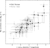Fig. 11.

Mass accretion rate vs. reference absolute V magnitude: comparison between the NLs of this paper and the classical novae in Selvelli & Gilmozzi (2019). They appear indistinguishable in terms of the correlation between Ṁ and $M_{V}^{ref}$ $M_{\mathrm{V}}^{\mathrm{ref}}$ .

10. Three NLs with shells as candidate old novae

A basic tenet of the hibernation theory for the evolution of CVs (see Shara et al. 1986, Livio 1992a,b) is that of a continuous cyclic evolution between CN, NL, hibernation, and Dwarf Nova (DN) states. The post-eruption phase of high Ṁ is of short duration (about a century or so) because it results from the post-eruption irradiation of the secondary by the hot WD. At this early stage the CV system will appear as a Nova-like.

Recent simulations of CVs evolution by Hillman et al. (2020) suggest a slightly different and more precise picture: newborn binaries, with longer P_orb (above the period gap) only alternate between nova and NL states during the first very few percent of the system life, then go through three states (nova-NL-DN) for the next ∼10%, finally entering a continuous cycle through all four states for the remaining ≲90% of their lifetimes.

One expectation with this scenario is that if NLs are indeed the remnants of novae exploded in recent centuries, one would expect to see nova shells around them. However, there is almost no evidence of this (nor around CVs in general, see Sahman et al. 2015; Schmidtobreick et al. 2015; Pagnotta & Zurek 2016). This problem has been recently addressed by Tappert et al. (2020) and Sahman & Dhillon (2022).

The only exceptions among NLs are V1315 Aql (Sahman et al. 2015, 2018), BZ Cam (Ellis et al. 1984; Krautter et al. 1987; Greiner et al. 2001; Godon et al. 2017; Hoffmann & Vogt 2020a) and the recently discovered NL V341 Ara (Castro Segura et al. 2021), which are associated with nebulosity. It is conceivable that these objects may have undergone nova explosions centuries ago.

A more precise estimate could be derived from the possible association of their eruption with some of the recorded observations of “guest stars” (GSs), mostly novae, described in ancient Chinese chronicles, see the compilations of historical observations by Clark & Stephenson (1977) and by Stephenson & Green (2009). These would provide invaluable input to assess the timescales of the changes in Ṁ after eruption but unfortunately it does not seem possible to associate these objects to any GSs.

For V1315 Aql, Sahman et al. (2018) derived a range of ages between 500 and 1200 years from a study of the shell structure, see Appendix A.2 for other details.

For BZ Cam and V341 Ara a possible association of their eruption time with some of the recorded observations of GSs has been recently suggested by Hoffmann & Vogt (2020a) and Castro Segura et al. (2021), respectively. Regrettably, we believe that these associations are also questionable, see Appendix A.2.

In any case the derived values of Ṁ show that these three NLs may have maintained high accretion rates (1 to 4 × 10⁻⁹ M_⊙ yr⁻¹) for centuries. These values would imply an inter-eruption interval of about 10⁴ − 10⁵ years if an accreted mass of about 10⁻⁴ − 10⁻⁵ M_⊙ is required to trigger the next eruption (this would agree with the expected inter-eruption interval in CNe).

If true, the above appears to be in agreement with the latest incarnation of the hibernation theory (Hillman et al. 2020) that predicts that recently formed CVs with long P_orb (i.e., above the period gap) just alternate between Nova and NL states and maintain high Ṁ. However, a disturbing piece of evidence in this context is that NLs inside the period gap also maintain high accretion rates (see Sect. 8.2).

11. Concluding remarks

The main purpose of this study was to determine $L_{disk}^{ref}$ $L_{\mathrm{disk}}^{\mathrm{ref}}$ and Ṁ for 42 NLs with UV spectra and Gaia EDR3 distances, and to explore whether this new input may improve our understanding of NLs. Regarding the points in Sect. 4 (the purpose of this work), we found the following:

Ṁ ∝ P_orb has been confirmed.
There is a different Ṁ for the same P_orb: despite the strong correlation of point 1, a scatter of almost one order of magnitude is present for Ṁ.
Ṁ drops for objects in the period gap, which is not seen. In fact, the nine objects in the gap have a similar if not higher Ṁ than those outside.
The claims of exceptionally high Ṁ in SW Sex stars are not confirmed: SW Sex stars have Ṁ indistinguishable from that of the other NL classes.
In comparing NLs’ Ṁ with that of old novae, we determined they are essentially identical.
In comparing Ṁ values derived in this paper with those from IUE data plus accretion disk models, we found they are not really comparable as the distances were from models rather than Gaia.

The most interesting result of this paper is that the NLs’ classes are essentially indistinguishable in terms of Ṁ and their correlation with various other quantities, such as the period, inclination, PL index, and absolute V magnitude. In fact, they are also indistinguishable in comparison to old novae (see Figs. 9 and 11), which is an indication that old novae and NLs are different phases of the same phenomenon. A consequence of the above is that a number of proxies for Ṁ have been identified and can be used to derive accretion rates from quantities that are easier to observe (e.g., P_orb, α, and $M_{V}^{ref}$ $M_V^{{\rm ref}}$ ), to within better than a factor of 2.

Our results are summarized below:

1. The continuum of NLs is well approximated by a power-law distribution with index α in the range −2.4 ≤ α ≤ −0.2. The observed optical magnitude is in very good agreement with the extrapolation of the UV power law to the optical range (see Fig. 4). These facts indicate that the disk dominates the UV and optical luminosities, and that the contributions by other sources are minor.

2. Despite rather large errors in the inclination i, the expected correlation between the continuum slope α and cos i is present (for the whole, UX and SW at p_H₀ < 10⁻⁴, see Fig. 3). Given these uncertainties it may not seem surprising that there is a large spread in α at any given inclination. However, some of the cases of high α and high i have some of the best determinations of both parameters, and may hint at different or distorted geometries of the disk (see Sect. 7.2).

3. NLs as a whole have a weighted mean log Ṁ = −8.61 ± 0.38 and a median log Ṁ = −8.63 (WLTO correction, M_WD = 0.76 M_⊙), with no difference between SW and nSW systems (see Table 5, bottom). This result is in stark contrast with previous claims of exceptionally high Ṁ in SW systems.

4. Nine NLs fall inside the period gap (as defined by Knigge 2006) but have an Ṁ similar to or slightly higher than that of objects above the gap. This result is confirmed by other observations (e.g., Dubus et al. 2018, see Fig. 7) and represents a major challenge to the common models of binary evolution and AMLs. In fact, these nine systems are in a semidetached configuration, contrary to the commonly accepted paradigm.

5. The SW class shows a large spread in Ṁ at a given P_orb (see Fig. 6), confirming previous findings by other methods.

6. In nSW systems there is a trend of higher Ṁ for longer periods (at p_H₀ < 10⁻⁴) that is not present in SW systems (Fig. 6).

7. The objects affected by the VY syndrome have a lower log Ṁ (weighted mean −8.80 ± 0.30, median −8.87) than the steady accretors’ UX systems (w.m. −8.4 ± 0.34, median −8.53; see the bottom of Table 5). A possible explanation is that not all VY objects were at maximum when observed (see Sect. 8.7).

8. The mass accretion rate Ṁ correlates with P_orb, α, and $M_{V}^{ref}$ $M_V^{{\rm ref}}$ , making them convenient proxies for Ṁ (Eqs. (10)–(12)). The strongest correlation (at p_H₀ < 10⁻⁶) is with $M_{V}^{ref}$ $M_V^{{\rm ref}}$ (see Fig. 9). Somewhat unexpectedly we found that an equally strong correlation exists between Ṁ and the uncorrected M_AAVSO (Eq. (13)).

9. The median log Ṁ of old novae (−8.61) is very similar to that of NLs as a class. Their weighted average log Ṁ is slightly lower (−8.37 ± 0.49) but well within the errors (see Fig. 10).

10. There is a possibility that the NL class definitions may need to be redefined or at least reassessed: (a) the histogram of the inclination distribution (Fig. 1) shows that the nSWs are segregated to lower inclinations (in fact there are none in eclipsing systems). This is most likely a selection effect, that is nSW objects appear to belong to a different class when seen at high inclination, and this may help explain the absence of correlation between α and i for this class; (b) it is intriguing that only VYs and nSWs (same objects) show PL indexes −1.1 > α > −1.6, although it is conceivable that this is just due to low number statistics; and (c) there is a period confinement of SWs and VYs, both peaking at P ≃ 3.9 h, which appears to us as a defining characteristic rather than a selection effect (see Fig. 1 and Table 2).

To conclude, we would like to reiterate that the combination of IUE UV spectra with Gaia EDR3 distances has proven to be a formidable tool to derive the critical parameters (de-reddened absolute disk luminosity and spectrum) necessary to determine the mass accretion rate in a consistent way. Without this input it would not have been possible to create a coherent sample of 42 objects or discover the correlations among physical properties and the similarities between NLs and classical novae.

Finally, we stress again that all quantities in this paper have associated error bars deriving from the propagation of the uncertainties from the basic parameters to the final values of the critical results. The coefficients of any correlations among quantities also have associated uncertainties. We believe that this is an important aspect of the study, as it shows both the limits and the accuracy of our results.

¹

https://web.archive.org/web/20180817023122/https://www.dwhoard.com/biglist

²

Specifically numpy, see www.numpy.org and unumpy-uncertainties, and http://pythonhosted.org/uncertainties/

Acknowledgments

This work is based on INES data from the IUE satellite (http://sdc.cab.inta-csic.es/ines/) and on data from the European Space Agency (ESA) mission Gaia (https://www.cosmos.esa.int/gaia), processed by the Gaia Data Processing and Analysis Consortium (DPAC, https://www.cosmos.esa.int/web/gaia/dpac/consortium). Funding for the DPAC has been provided by national institutions, in particular the institutions participating in the Gaia Multilateral Agreement. We wish to thank and commend the AAVSO for their excellent photometric work on variable stars: their results have been of invaluable help to us in this paper. We thank Elena Mason and Antonio Bianchini for fruitful discussions, and the anonymous referee for helpful and meticulous comments and suggestions.

References

Andronov, N., Pinsonneault, M., & Sills, A. 2003, ApJ, 582, 358 [NASA ADS] [CrossRef] [Google Scholar]
Araujo-Betancor, S., Knigge, C., Long, K. S., et al. 2003, ApJ, 583, 437 [NASA ADS] [CrossRef] [Google Scholar]
Asuero, A. G., Sayago, A., & Gonzalez, A. 2006, Crit. Rev. Anal. Chem, 36, 41 [CrossRef] [Google Scholar]
Bailer-Jones, C. A. L. 2015, PASP, 127, 994 [Google Scholar]
Bailer-Jones, C. A. L., Rybizki, J., Fouesneau, M., et al. 2018, AJ, 156, 58 [NASA ADS] [CrossRef] [Google Scholar]
Ballouz, R.-L., & Sion, E. M. 2009, ApJ, 697, 1717 [NASA ADS] [CrossRef] [Google Scholar]
Baptista, R., Jablonski, F. J., Cieslinski, D., et al. 1993, ApJ, 406, L67 [NASA ADS] [CrossRef] [Google Scholar]
Baptista, R., Horne, K., Hilditch, R. W., et al. 1995, ApJ, 448, 395 [NASA ADS] [CrossRef] [Google Scholar]
Beuermann, K., Thorstensen, J. R., Schwope, A. D., et al. 1992, A&A, 256, 442 [NASA ADS] [Google Scholar]
Bisol, A. C., Godon, P., & Sion, E. M. 2012, PASP, 124, 158 [NASA ADS] [CrossRef] [Google Scholar]
Bond, H. E., & Miszalski, B. 2018, PASP, 130, 094201 [NASA ADS] [CrossRef] [Google Scholar]
Borges, B. W., & Baptista, R. 2005, Magnetic Fields in the Universe: From Laboratory and Stars to Primordial Structures, 784, 685 [NASA ADS] [CrossRef] [Google Scholar]
Boyd, D. 2009, British Astronomical Association Variable Star Section Circular, 142 [Google Scholar]
Bruch, A. 2021, MNRAS, 503, 953 [NASA ADS] [CrossRef] [Google Scholar]
Bruch, A., & Diaz, M. P. 2017, New A, 50, 109 [NASA ADS] [CrossRef] [Google Scholar]
Cannizzo, J. K. 1998, ApJ, 493, 426 [NASA ADS] [CrossRef] [Google Scholar]
Capitanio, L., Lallement, R., Vergely, J. L., et al. 2017, A&A, 606, A65 [NASA ADS] [CrossRef] [EDP Sciences] [Google Scholar]
Cardelli, J. A., Clayton, G. C., & Mathis, J. S. 1989, ApJ, 345, 245 [Google Scholar]
Castro Segura, N., Knigge, C., Acosta-Pulido, J. A., et al. 2021, MNRAS, 501, 1951 [NASA ADS] [CrossRef] [Google Scholar]
Clark, D. H., & Stephenson, F. R. 1977, Oxford [Eng.] (New York: Pergamon Press) [Google Scholar]
Cordova, F. A., & Mason, K. O. 1985, ApJ, 290, 671 [NASA ADS] [CrossRef] [Google Scholar]
Cordova, F. A., & Howarth, I. D. 1987, Exploring the Universe with the IUE Satellite, 129, 395 [NASA ADS] [CrossRef] [Google Scholar]
Dai, Z.-B., Qian, S.-B., Fernández Lajús, E., et al. 2010, MNRAS, 409, 1195 [CrossRef] [Google Scholar]
D’Antona, F., Mazzitelli, I., & Ritter, H. 1989, A&A, 225, 391 [Google Scholar]
Davis, P. J., Kolb, U., Willems, B., et al. 2008, MNRAS, 389, 1563 [NASA ADS] [CrossRef] [Google Scholar]
Deming, W. E. 1943, Statistical adjustment of data, Wiley, NY (DoverPublications edition, 1985) [Google Scholar]
Dhillon, V. S. 1996, in IAU Colloq. 158: Cataclysmic Variables and Related Objects, 208, 3 [NASA ADS] [CrossRef] [Google Scholar]
Dhillon, V. S., Marsh, T. R., & Jones, D. H. P. 1991, MNRAS, 252, 342 [NASA ADS] [CrossRef] [Google Scholar]
Dhillon, V. S., Jones, D. H. P., Marsh, T. R., et al. 1992, MNRAS, 258, 225 [NASA ADS] [CrossRef] [Google Scholar]
Dhillon, V. S., Marsh, T. R., & Jones, D. H. P. 1997, MNRAS, 291, 694 [Google Scholar]
Dhillon, V. S., Smith, D. A., & Marsh, T. R. 2013, MNRAS, 428, 3559 [Google Scholar]
Diaz, M. P., & Hubeny, I. 1999, ApJ, 523, 786 [NASA ADS] [CrossRef] [Google Scholar]
Donati, J. F. 2006, 36th COSPAR Scientific Assembly [Google Scholar]
Downes, R. A., Webbink, R. F., Shara, M. M., et al. 2001, PASP, 113, 764 [Google Scholar]
Downes, R. A., Webbink, R. F., Shara, M. M., et al. 2006, VizieR Online Data Catalog: V/123A [Google Scholar]
Draper, N. R. 1991, Conference on Applied Statistics in Agriculture, 1 [Google Scholar]
Drew, J. E., Hartley, L. E., Long, K. S., et al. 2003, MNRAS, 338, 401 [NASA ADS] [CrossRef] [Google Scholar]
Dubus, G., Otulakowska-Hypka, M., & Lasota, J.-P. 2018, A&A, 617, A26 [NASA ADS] [CrossRef] [EDP Sciences] [Google Scholar]
Eggleton, P. 2011, 2011, Evolutionary Processes in Binary and Multiple Stars, by Peter Eggleton, Cambridge (UK: Cambridge University Press) [Google Scholar]
Eggleton, P., Mitton, S., & Whelan, J. 1976, Structure and Evolution of Close Binary Systems, 73 [Google Scholar]
Ellis, G. L., Grayson, E. T., & Bond, H. E. 1984, PASP, 96, 283 [NASA ADS] [CrossRef] [Google Scholar]
El-Badry, K., Conroy, C., Fuller, J., et al. 2022, MNRAS, 517, 4916 [NASA ADS] [CrossRef] [Google Scholar]
Faulkner, J. 1971, ApJ, 170, L99 [NASA ADS] [CrossRef] [Google Scholar]
Feiden, G. A., Skidmore, K., & Jao, W.-C. 2021, ApJ, 907, 53 [NASA ADS] [CrossRef] [Google Scholar]
Frank, J., & King, A. R. 1981, MNRAS, 195, 227 [NASA ADS] [CrossRef] [Google Scholar]
Frank, J., King, A., & Raine, D. J. 2002, Accretion Power in Astrophysics (Cambridge, UK: Cambridge University Press), 398 [Google Scholar]
Froning, C. S., Long, K. S., & Baptista, R. 2003, AJ, 126, 964 [NASA ADS] [CrossRef] [Google Scholar]
Froning, C. S., Long, K. S., Szkody, P., et al. 2004, Rev. Mex. Astron. Astrofis. Conf. Ser., 20, 251 [NASA ADS] [Google Scholar]
Froning, C. S., Long, K. S., Gänsicke, B., et al. 2012, ApJS, 199, 7 [NASA ADS] [CrossRef] [Google Scholar]
Gänsicke, B. T. 2004, Rev. Mex. Astron. Astrofis. Conf. Ser., 20, 152 [Google Scholar]
Gänsicke, B. T., & Koester, D. 1999, A&A, 346, 151 [Google Scholar]
Gaia Collaboration (Brown, A. G. A., et al.) 2021, A&A, 649, A1 [NASA ADS] [CrossRef] [EDP Sciences] [Google Scholar]
Garraffo, C., Drake, J. J., & Cohen, O. 2016, A&A, 595, A110 [NASA ADS] [CrossRef] [EDP Sciences] [Google Scholar]
Garraffo, C., Drake, J. J., Alvarado-Gomez, J. D., et al. 2018, ApJ, 868, 60 [NASA ADS] [CrossRef] [Google Scholar]
Gilliland, R. L., & Phillips, M. M. 1982, ApJ, 261, 617 [NASA ADS] [CrossRef] [Google Scholar]
Gilmozzi, R., & Selvelli, P. 2007, A&A, 461, 593 [NASA ADS] [CrossRef] [EDP Sciences] [Google Scholar]
Godon, P., Sion, E. M., Balman, Ş., et al. 2017, ApJ, 846, 52 [NASA ADS] [CrossRef] [Google Scholar]
González-Riestra, R., Cassatella, A., & Wamsteker, W. 2001, A&A, 373, 730 [NASA ADS] [CrossRef] [EDP Sciences] [Google Scholar]
Greiner, J., Tovmassian, G. H., Di Stefano, R., et al. 1999, A&A, 343, 183 [NASA ADS] [Google Scholar]
Greiner, J., Tovmassian, G., Orio, M., et al. 2001, A&A, 376, 1031 [NASA ADS] [CrossRef] [EDP Sciences] [Google Scholar]
Groot, P. J., Rutten, R. G. M., & van Paradijs, J. 2004, A&A, 417, 283 [NASA ADS] [CrossRef] [EDP Sciences] [Google Scholar]
Hameury, J.-M. 1994, IAU Colloq. 147: The Equation of State in Astrophysics, 420 [CrossRef] [Google Scholar]
Hameury, J.-M., & Lasota, J.-P. 2002, A&A, 394, 231 [NASA ADS] [CrossRef] [EDP Sciences] [Google Scholar]
Hamilton, R. T., Urban, J. A., Sion, E. M., et al. 2007, ApJ, 667, 1139 [NASA ADS] [CrossRef] [Google Scholar]
Hellier, C., & Naylor, T. 1998, MNRAS, 295, L50 [NASA ADS] [CrossRef] [Google Scholar]
Hellier, C., O’Donoghue, D., Buckley, D., et al. 1990, MNRAS, 242, 32 [Google Scholar]
Hellier, C., Ringwald, F. A., & Robinson, E. L. 1994, A&A, 289, 148 [NASA ADS] [Google Scholar]
Hessman, F. V. 1988, A&AS, 72, 515 [NASA ADS] [Google Scholar]
Hillman, Y., Shara, M. M., Prialnik, D., et al. 2020, Nat. Astron., 4, 886 [CrossRef] [Google Scholar]
Ho, P. Y. 1962, Vistas Astron., 5, 127 [NASA ADS] [CrossRef] [Google Scholar]
Hoard, D. W., & Szkody, P. 1996, ApJ, 470, 1052 [NASA ADS] [CrossRef] [Google Scholar]
Hoard, D. W., & Szkody, P. 1997, ApJ, 481, 433 [Google Scholar]
Hoard, D. W., Szkody, P., Still, M. D., et al. 1998, MNRAS, 294, 689 [NASA ADS] [CrossRef] [Google Scholar]
Hoard, D. W., Thorstensen, J. R., & Szkody, P. 2000, ApJ, 537, 936 [NASA ADS] [CrossRef] [Google Scholar]
Hoard, D. W., Wachter, S., Clark, L. L., et al. 2002, ApJ, 565, 511 [NASA ADS] [CrossRef] [Google Scholar]
Hoard, D. W., Szkody, P., Froning, C. S., et al. 2003, AJ, 126, 2473 [NASA ADS] [CrossRef] [Google Scholar]
Hoard, D. W., Lu, T.-N., Knigge, C., et al. 2010, AJ, 140, 1313 [NASA ADS] [CrossRef] [Google Scholar]
Hoard, D. W., Long, K. S., Howell, S. B., et al. 2014, ApJ, 786, 68 [NASA ADS] [CrossRef] [Google Scholar]
Hoffmann, S. M., & Vogt, N. 2020a, MNRAS, 497, 1419 [CrossRef] [Google Scholar]
Hoffmann, S. M., Vogt, N., & Protte, P. 2020b, Astron. Nachr., 341, 79 [NASA ADS] [CrossRef] [Google Scholar]
Honeycutt, R. K., Schlegel, E. M., & Kaitchuck, R. H. 1986, ApJ, 302, 388 [NASA ADS] [CrossRef] [Google Scholar]
Honeycutt, R. K., Livio, M., & Robertson, J. W. 1993, PASP, 105, 922 [NASA ADS] [CrossRef] [Google Scholar]
Horne, K., & Stiening, R. F. 1985, MNRAS, 216, 933 [NASA ADS] [Google Scholar]
Howell, S. B., & Mason, E. 2018, AJ, 156, 198 [NASA ADS] [CrossRef] [Google Scholar]
Howell, S. B., Nelson, L. A., & Rappaport, S. 2001, ApJ, 550, 897 [Google Scholar]
Hsi, T.-T. 1957, Smithsonian Contributions to Astrophysics, 2, 109 [NASA ADS] [Google Scholar]
Huber, M. E., Howell, S. B., Ciardi, D. R., et al. 1998, PASP, 110, 784 [NASA ADS] [CrossRef] [Google Scholar]
Hutchings, J. B., Link, R., & Crampton, D. 1983, PASP, 95, 264 [NASA ADS] [CrossRef] [Google Scholar]
Hutchings, J. B., & Cowley, A. P. 1984, PASP, 96, 559 [NASA ADS] [CrossRef] [Google Scholar]
Ihn, T. 2016, https://vp.phys.ethz.ch/DataAnalysis/pdf/14Nov2016.pdf [Google Scholar]
Jameson, R. F., King, A. R., & Sherrington, M. R. 1982, MNRAS, 200, 455 [NASA ADS] [CrossRef] [Google Scholar]
Jao, W.-C., Henry, T. J., Gies, D. R., et al. 2018, ApJ, 861, L11 [NASA ADS] [CrossRef] [Google Scholar]
Jones, B. F., Fischer, D. A., & Stauffer, J. R. 1996, AJ, 112, 1562 [NASA ADS] [CrossRef] [Google Scholar]
Kafka, S., & Honeycutt, R. K. 2005, AJ, 130, 742 [NASA ADS] [CrossRef] [Google Scholar]
Kafka, S., & Honeycutt, R. K. 2006, AJ, 132, 1517 [NASA ADS] [CrossRef] [Google Scholar]
Kafka, S., Anderson, R., & Honeycutt, R. K. 2008, AJ, 135, 1649 [NASA ADS] [CrossRef] [Google Scholar]
Kelly, B. D., Kilkenny, D., & Cooke, J. A. 1981, MNRAS, 196, 91P [NASA ADS] [CrossRef] [Google Scholar]
King, A. R. 1988, QJRAS, 29, 1 [NASA ADS] [Google Scholar]
Knigge, C. 2006, MNRAS, 373, 484 [NASA ADS] [CrossRef] [Google Scholar]
Knigge, C. 2011, Evol. Compact Binaries, 447, 3 [NASA ADS] [Google Scholar]
Knigge, C., Baraffe, I., & Patterson, J. 2011, ApJS, 194, 28 [Google Scholar]
Knigge, C., & Drew, J. E. 1997, ApJ, 486, 445 [CrossRef] [Google Scholar]
Knigge, C., Long, K. S., Wade, R. A., et al. 1998, ApJ, 499, 414 [NASA ADS] [CrossRef] [Google Scholar]
Knigge, C. 2011, vol. Compact Binaries, 447, 3 [NASA ADS] [Google Scholar]
Kolb, U. 1996, IAU Colloq. 158: Cataclysmic Variables and Related Objects, 208, 433 [NASA ADS] [CrossRef] [Google Scholar]
Kolb, U. 2001, The Influence of Binaries on Stellar Population Studies, 264, 321 [NASA ADS] [CrossRef] [Google Scholar]
Kolb, U., & Ritter, H. 1992, A&A, 254, 213 [NASA ADS] [Google Scholar]
Krautter, J., Klaas, U., & Radons, G. 1987, A&A, 181, 373 [NASA ADS] [Google Scholar]
La Dous, C. 1989, A&A, 211, 131 [NASA ADS] [Google Scholar]
La Dous, C. 1991, A&A, 252, 100 [NASA ADS] [Google Scholar]
La Dous, C. 1993, Cataclysmic Variables Related Phys., 10, 39 [Google Scholar]
La Dous, C. 1994, Space Sci. Rev., 67, 1 [CrossRef] [Google Scholar]
Linnell, A. P., Szkody, P., Gänsicke, B., et al. 2005, ApJ, 624, 923 [NASA ADS] [CrossRef] [Google Scholar]
Linnell, A. P., Godon, P., Hubeny, I., et al. 2008, ApJ, 676, 1226 [NASA ADS] [CrossRef] [Google Scholar]
Linnell, A. P., Godon, P., Hubeny, I., et al. 2009, ApJ, 703, 1839 [NASA ADS] [CrossRef] [Google Scholar]
Livio, M. 1992a, Cataclysmic Variable Stars, 29, 4 [NASA ADS] [Google Scholar]
Livio, M. 1992b, Cataclysmic Variable Stars, 29, 269 [NASA ADS] [Google Scholar]
Livio, M. 1994, Saas-Fee Advanced Course 22: Interacting Binaries, 155 [Google Scholar]
Long, K. S., Wade, R. A., Blair, W. P., et al. 1994, ApJ, 426, 704 [NASA ADS] [CrossRef] [Google Scholar]
Luri, X., Brown, A. G. A., Sarro, L. M., et al. 2018, A&A, 616, A9 [NASA ADS] [CrossRef] [EDP Sciences] [Google Scholar]
Martínez-Pais, I. G., Martín-Hernández, N. L., Casares, J., et al. 2000, ApJ, 538, 315 [CrossRef] [Google Scholar]
Meyer, F., & Meyer-Hofmeister, E. 1984, A&A, 132, 143 [NASA ADS] [Google Scholar]
Mizusawa, T., Merritt, J., Ballouz, R.-L., et al. 2010, PASP, 122, 299 [NASA ADS] [CrossRef] [Google Scholar]
Morales, J. C., Ribas, I., Giménez, Á., et al. 2022, Galaxies, 10, 98 [NASA ADS] [CrossRef] [Google Scholar]
Morrell, S., & Naylor, T. 2019, MNRAS, 489, 2615 [NASA ADS] [CrossRef] [Google Scholar]
Neustroev, V. V., Suleimanov, V. F., Borisov, N. V., et al. 2011, MNRAS, 410, 963 [CrossRef] [Google Scholar]
Nickiforov, M. G. 2010, Bulgarian. Astron. J., 13, 116 [NASA ADS] [Google Scholar]
Noebauer, U. M., Long, K. S., Sim, S. A., et al. 2010, ApJ, 719, 1932 [NASA ADS] [CrossRef] [Google Scholar]
North, R. C., Marsh, T. R., Kolb, U., et al. 2002, MNRAS, 337, 1215 [NASA ADS] [CrossRef] [Google Scholar]
Norton, A. J., Beardmore, A. P., Retter, A., et al. 2000, MNRAS, 312, 362 [NASA ADS] [CrossRef] [Google Scholar]
Oliveira, A. S., Lima, H. J. F., Steiner, J. E., et al. 2014, MNRAS, 444, 2692 [Google Scholar]
Orosz, J. A., & Wade, R. A. 2003, ApJ, 593, 1032 [NASA ADS] [CrossRef] [Google Scholar]
Osaki, Y. 1974, PASJ, 26, 429 [NASA ADS] [Google Scholar]
Paczynski, B., & Schwarzenberg-Czerny, A. 1980, Acta Astron., 30, 127 [NASA ADS] [Google Scholar]
Paczynski, B., & Sienkiewicz, R. 1981, ApJ, 248, L27 [NASA ADS] [CrossRef] [Google Scholar]
Paczynski, B., & Sienkiewicz, R. 1983, ApJ, 268, 825 [NASA ADS] [CrossRef] [Google Scholar]
Pagnotta, A., & Zurek, D. 2016, MNRAS, 458, 1833 [NASA ADS] [CrossRef] [Google Scholar]
Pala, A. F., Gänsicke, B. T., Townsley, D., et al. 2017, MNRAS, 466, 2855 [NASA ADS] [CrossRef] [Google Scholar]
Pala, A. F., Gänsicke, B. T., Belloni, D., et al. 2022, MNRAS, 510, 6110 [NASA ADS] [CrossRef] [Google Scholar]
Parsons, S. G., Gänsicke, B. T., Marsh, T. R., et al. 2018, MNRAS, 481, 1083 [Google Scholar]
Patterson, J. 1984, ApJS, 54, 443 [NASA ADS] [CrossRef] [Google Scholar]
Patterson, J. 2011, MNRAS, 411, 2695 [NASA ADS] [CrossRef] [Google Scholar]
Patterson, J., Fenton, W. H., Thorstensen, J. R., et al. 2002, PASP, 114, 1364 [Google Scholar]
Patterson, J., Kemp, J., Harvey, D. A., et al. 2005, PASP, 117, 1204 [Google Scholar]
Perryman, M., & Zioutas, K. 2022, Symmetry, 14, 721 [NASA ADS] [CrossRef] [Google Scholar]
Petterson, J. A. 1980, ApJ, 241, 247 [NASA ADS] [CrossRef] [Google Scholar]
Politano, M. 1990, Accretion-Powered Compact Binaries, 421 [Google Scholar]
Politano, M., Livio, M., & Truran, J. W. 1990, IAU Colloq. 122: Physics of Classical Novae, 386 [NASA ADS] [CrossRef] [Google Scholar]
Poole, T., Mason, K. O., Ramsay, G., et al. 2003, MNRAS, 340, 499 [NASA ADS] [CrossRef] [Google Scholar]
Postnov, K. A., & Yungelson, L. R. 2014, Liv. Rev. Relativity, 17, 3 [NASA ADS] [CrossRef] [Google Scholar]
Prinja, R. K., & Rosen, R. 1995, MNRAS, 273, 461 [CrossRef] [Google Scholar]
Prinja, R. K., Knigge, C., Witherick, D. K., et al. 2004, MNRAS, 355, 137 [NASA ADS] [CrossRef] [Google Scholar]
Puebla, R. E., Diaz, M. P., & Hubeny, I. 2007, AJ, 134, 1923 [Google Scholar]
Quenouille, M. H. 1949, Approximate use of correlation in timeseries, ISO4, Series B, 11:18, 84 [Google Scholar]
Ramsay, G., Wheatley, P. J., Norton, A. J., et al. 2008, MNRAS, 387, 1157 [NASA ADS] [CrossRef] [Google Scholar]
Ramsay, G., Schreiber, M. R., Gänsicke, B. T., et al. 2017, A&A, 604, A107 [NASA ADS] [CrossRef] [EDP Sciences] [Google Scholar]
Rappaport, S., Verbunt, F., & Joss, P. C. 1983, ApJ, 275, 713 [Google Scholar]
Ringwald, F. A., & Naylor, T. 1998, AJ, 115, 286 [NASA ADS] [CrossRef] [Google Scholar]
Ritter, H. 1984, A&AS, 57, 385 [NASA ADS] [Google Scholar]
Ritter, H. 1990, IAU Colloq. 122: Physics of Classical Novae, 313 [Google Scholar]
Ritter, H. 1991, High Energy Astrophysics: Compact Stars and Active Galaxies, 107 [Google Scholar]
Ritter, H. 2012, Mem. Soc. Astron. It., 83, 505 [NASA ADS] [Google Scholar]
Ritter, H., & Kolb, U. 2011, VizieR Online Data Catalog, B/cb [Google Scholar]
Ritter, H., Politano, M., Livio, M., et al. 1991, ApJ, 376, 177 [NASA ADS] [CrossRef] [Google Scholar]
Rodríguez-Gil, P., Casares, J., Dhillon, V. S., et al. 2000, A&A, 355, 181 [Google Scholar]
Rodríguez-Gil, P., Schmidtobreick, L., & Gänsicke, B. T. 2007a, MNRAS, 374, 1359 [NASA ADS] [CrossRef] [Google Scholar]
Rodríguez-Gil, P., Gänsicke, B. T., Hagen, H.-J., et al. 2007b, MNRAS, 377, 1747 [NASA ADS] [CrossRef] [Google Scholar]
Rodríguez-Gil, P., Schmidtobreick, L., Long, K. S., et al. 2012, Mem. Soc. Astron. It., 83, 602 [Google Scholar]
Rodríguez-Gil, P., Shahbaz, T., Torres, M. A. P., et al. 2020, MNRAS, 494, 425 [CrossRef] [Google Scholar]
Rodríguez-Pascual, P. M., González-Riestra, R., Schartel, N., et al. 1999, A&AS, 139, 183 [NASA ADS] [CrossRef] [EDP Sciences] [Google Scholar]
Rolfe, D. J., Haswell, C. A., & Patterson, J. 2000, MNRAS, 317, 759 [NASA ADS] [CrossRef] [Google Scholar]
Rude, G. D., & Ringwald, F. A. 2012, New A, 17, 453 [NASA ADS] [CrossRef] [Google Scholar]
Rutten, R. G. M., van Paradijs, J., & Tinbergen, J. 1992, A&A, 260, 213 [NASA ADS] [Google Scholar]
Sahman, D. I., & Dhillon, V. S. 2022, MNRAS, 510, 4180 [CrossRef] [Google Scholar]
Sahman, D. I., Dhillon, V. S., Knigge, C., et al. 2015, MNRAS, 451, 2863 [NASA ADS] [CrossRef] [Google Scholar]
Sahman, D. I., Dhillon, V. S., Littlefair, S. P., et al. 2018, MNRAS, 477, 4483 [NASA ADS] [CrossRef] [Google Scholar]
Schmidtke, P. C., Ciudin, G. A., Indlekofer, U. R., et al. 2002, The Physics of Cataclysmic Variables and Related Objects, 261, 539 [NASA ADS] [Google Scholar]
Schmidtobreick, L. 2017, ArXiv e-prints [arXiv:1705.09332] [Google Scholar]
Schmidtobreick, L., & Tappert, C. 2015, Acta Polytechnica CTU Proceedings, 2, 188 [NASA ADS] [CrossRef] [Google Scholar]
Schmidtobreick, L., Rodríguez-Gil, P., & Gänsicke, B. T. 2012, Mem. Soc. Astron. It., 83, 610 [NASA ADS] [Google Scholar]
Schmidtobreick, L., Shara, M., Tappert, C., et al. 2015, MNRAS, 449, 2215 [NASA ADS] [CrossRef] [Google Scholar]
Selvelli, P., & Gilmozzi, R. 2019, A&A, 622, A186 [NASA ADS] [CrossRef] [EDP Sciences] [Google Scholar]
Shafter, A. W. 1983, Ph.D. Thesis, USA [Google Scholar]
Shafter, A. W. 1985, AJ, 90, 643 [NASA ADS] [CrossRef] [Google Scholar]
Shafter, A. W. 1992, ApJ, 394, 268 [NASA ADS] [CrossRef] [Google Scholar]
Shafter, A. W., Wheeler, J. C., & Cannizzo, J. K. 1986, ApJ, 305, 261 [NASA ADS] [CrossRef] [Google Scholar]
Shara, M. M., Livio, M., Moffat, A. F. J., et al. 1986, ApJ, 311, 163 [Google Scholar]
Shugarov, S. Y., Katysheva, N. A., & Kroll, P. 2007, 15th European Workshop on White Dwarfs, 372, 515 [Google Scholar]
Šimon, V. 2017, Astron. Nachr., 338, 696 [CrossRef] [Google Scholar]
Šimon, V., Polášek, C., Štrobl, J., et al. 2012, A&A, 540, A15 [NASA ADS] [CrossRef] [EDP Sciences] [Google Scholar]
Sion, E. M., & Godon, P. 2022, Galaxies, 10, 43 [NASA ADS] [CrossRef] [Google Scholar]
Sion, E. M., Mizusawa, T., & Ballouz, R.-L. 2009, J. Phys. Conf. Ser., 172, 012039P [NASA ADS] [CrossRef] [Google Scholar]
Skumanich, A. 1972, ApJ, 171, 565 [Google Scholar]
Smak, J. 1984, PASP, 96, 5 [NASA ADS] [CrossRef] [Google Scholar]
Smak, J. 2002, Acta Astron., 52, 429 [NASA ADS] [Google Scholar]
Smak, J. 2019, Acta Astron., 69, 79 [NASA ADS] [Google Scholar]
Smith, R. C. 2007, ArXiv e-prints [arXiv:astro-ph/0701654] [Google Scholar]
Smith, D. A., Dhillon, V. S., & Marsh, T. R. 1998, MNRAS, 296, 465 [NASA ADS] [CrossRef] [Google Scholar]
Spruit, H. C., & Ritter, H. 1983, A&A, 124, 267 [NASA ADS] [Google Scholar]
Spruit, H. C., & Taam, R. E. 2001, ApJ, 548, 900 [NASA ADS] [CrossRef] [Google Scholar]
Steiner, J. E., & Diaz, M. P. 1998, PASP, 110, 276 [NASA ADS] [CrossRef] [Google Scholar]
Stephenson, F. R., & Green, D. A. 2009, J. History Astron., 40, 31 [Google Scholar]
Stickland, D. J., Kelly, B. D., Cooke, J. A., et al. 1984, MNRAS, 206, 819 [NASA ADS] [CrossRef] [Google Scholar]
Szkody, P., & Gaensicke, B. T. 2012, JAAVSO, 40, 563 [NASA ADS] [Google Scholar]
Szkody, P., & Shafter, A. W. 1983, PASP, 95, 509 [Google Scholar]
Taam, R. E., & Spruit, H. C. 1989, ApJ, 345, 972 [NASA ADS] [CrossRef] [Google Scholar]
Tappert, C., Hanuschik, R. W., & Wargau, W. F. 1998, Astronomische Gesellschaft Abstract Series [Google Scholar]
Tappert, C., Vogt, N., Ederoclite, A., et al. 2020, A&A, 641, A122 [NASA ADS] [CrossRef] [EDP Sciences] [Google Scholar]
Taylor, C. J., Thorstensen, J. R., & Patterson, J. 1999, PASP, 111, 184 [NASA ADS] [CrossRef] [Google Scholar]
Thomas, N. L., Norton, A. J., Pollacco, D., et al. 2010, A&A, 514, A30 [NASA ADS] [CrossRef] [EDP Sciences] [Google Scholar]
Thoroughgood, T. D., Dhillon, V. S., Watson, C. A., et al. 2004, MNRAS, 353, 1135 [Google Scholar]
Thorstensen, J. R., Ringwald, F. A., Wade, R. A., et al. 1991, AJ, 102, 272 [NASA ADS] [CrossRef] [Google Scholar]
Townsley, D. M., & Gänsicke, B. T. 2009, ApJ, 693, 1007 [Google Scholar]
Truran, J. W., & Livio, M. 1986, ApJ, 308, 721 [NASA ADS] [CrossRef] [Google Scholar]
Tukey, J. W. 1958, Bias and confidence in not quite large samples (Ann.Math. Stat. 29, 614 1958) [Google Scholar]
Vande Putte, D., Smith, R. C., Hawkins, N. A., et al. 2003, MNRAS, 342, 151 [NASA ADS] [CrossRef] [Google Scholar]
Verbunt, F. 1987, A&AS, 71, 339 [Google Scholar]
Verbunt, F. 1991, Adv. Space Res., 11, 57 [NASA ADS] [CrossRef] [Google Scholar]
Verbunt, F. 1997, MNRAS, 290, L55 [CrossRef] [Google Scholar]
Verbunt, F., & Zwaan, C. 1981, A&A, 100, L7 [NASA ADS] [Google Scholar]
Wade, R. A. 1988, ApJ, 335, 394 [NASA ADS] [CrossRef] [Google Scholar]
Wade, R. A., & Hubeny, I. 1998, ApJ, 509, 350 [NASA ADS] [CrossRef] [Google Scholar]
Warner, B. 1986, MNRAS, 222, 11 [NASA ADS] [Google Scholar]
Warner, B. 1987, MNRAS, 227, 23 [NASA ADS] [Google Scholar]
Warner, B. 1995, Camb. Astrophys. Ser., 28 [Google Scholar]
Warner, B. 2000, New Astron. Rev., 44, 3 [NASA ADS] [CrossRef] [Google Scholar]
Webbink, R. F., Livio, M., Truran, J. W., et al. 1987, ApJ, 314, 653 [NASA ADS] [CrossRef] [Google Scholar]
Wenzel, W., Banny, M. I., Bannyj, M. I., et al. 1988, Zentralinstitut fuer Astrophysik Sternwarte Sonneberg Mitteilungen ueber Veraenderliche Sterne, 11, 141 [NASA ADS] [Google Scholar]
Willems, B., Kolb, U., Sandquist, E. L., et al. 2005, ApJ, 635, 1263 [NASA ADS] [CrossRef] [Google Scholar]
Willems, B., Taam, R. E., Kolb, U., et al. 2007, ApJ, 657, 465 [NASA ADS] [CrossRef] [Google Scholar]
Wolfe, A., Sion, E. M., & Bond, H. E. 2013, AJ, 145, 168 [NASA ADS] [CrossRef] [Google Scholar]
Woudt, P. A., Warner, B., de Budé, D., et al. 2012, MNRAS, 421, 2414 [NASA ADS] [CrossRef] [Google Scholar]
Xi, Z., & Po, S. 1966, in Ancient Novae and Supernovae Recorded in the Annals of China, Korea, and Japan and Their Significance in Radioastronomy (Washington: National Aeronautics and Space Administration) [Google Scholar]
Xi, Z.-Z., Po, S.-J., & Yang, K. S. 1966, Science, 154, 597 [NASA ADS] [CrossRef] [Google Scholar]
Xu, Z., Pankenier, D. W., & Jian, Y. 2000, East Asian Archaeoastronomy : Historical Records of Astronomical Observations of China, Japan, and Korea, Earth Space Institute (ESI) book series (Amsterdam: Gordon and Breach), 5, 8 [Google Scholar]
Yau, K. K. C. 1988, Ph.D. Thesis, UK [Google Scholar]
Young, P., & Schneider, D. P. 1981, ApJ, 247, 960 [NASA ADS] [CrossRef] [Google Scholar]
Zorotovic, M., & Schreiber, M. R. 2020, Adv. Space Res., 66, 1080 [NASA ADS] [CrossRef] [Google Scholar]
Zorotovic, M., Schreiber, M. R., Parsons, S. G., et al. 2016, MNRAS, 457, 3867 [Google Scholar]

Appendix A: Comments on some individual NLs

A.1. Objects with uncertain inclination

Six of the NLs in our sample have discordant i values in the literature.

WX Ari: Warner (1995) gives i ≤ 65 while Ritter & Kolb (2011) and La Dous (1991) give i ∼ 74. Rodríguez-Gil et al. (2000) derive i ∼ 74 from the presence of a very shallow eclipse (0.15 mag) in the R-band. The same value is reported by Puebla et al. (2007) and by Godon et al. (2017) while Ballouz & Sion (2009) give i = 60. However, Hoard et al. (2010) indicates "low-moderate inclination;" Beuermann et al. (1992) and Hellier et al. (1994) mention the absence of eclipses and suggest low i. We have used i = 65 ± 10 and determined α = −0.73 ± 0.06 (note that the PL fits are done on the de-reddened spectra, without any correction for inclination).

QU Car: Ritter & Kolb (2011) give i = 60, but La Dous (1991) gives i < 60 as do Gilliland & Phillips (1982). Hoard et al. (2014) give a range 40−60, Bruch (2021) gives i = 50, Puebla et al. (2007) indicate a range 35 − 65. We have used i = 60 ± 4.

CM Del: A large uncertainty in i has been recently pointed out by Howell & Mason (2019). Shafter (1983, Thesis, p. 104) gives high i with large error: i = 73 ± 47, a value later reported by Ritter & Kolb (2011), La Dous (1991) and Puebla et al. (2007) who also give the range i ∼ 60 − 85, while Ballouz & Sion 2009 give i = 75. Warner (1995) gives contradictory values: in pp. 218, 225 he suggests i = 30 referring to Shafter’s 1983 thesis (that actually gives 73 ± 47), to Shafter (1985), who does not actually give any value for the inclination, and to Szkody & Shafter (1983), who only mention that there is no evidence of high i. To make the situation even less clear, Warner (Warner 1995, p.234) includes CM Del within high inclination NLs. Given that there are no eclipses reported, the inclination should be less than ∼65 deg. We have used i = 57 ± 17

RZ Gru: Ritter & Kolb (2011) and La Dous (1991) do not provide any value for i. We have used i = 61 ± 7, from Kelly et al. (1981) and the synthetic spectral fitting by Bisol et al. (2012). However, a low inclination was suggested by Stickland et al. (1984) from IUE data, by Tappert et al. (1998) from the presence of a sharp Hα line, and by Froning et al. (2012) from FUSE data. Note that IUE spectra show the presence of 3 P Cyg profiles for NV 1240, SiIV 1400, and CIV 1550, with deep absorption components.

V442 Oph: Ritter & Kolb (2011), La Dous (1991) and Puebla et al. (2007) give i = 67 ± 27, Ballouz & Sion (2009)i = 75, Warner (1995)i = 60, Hoard et al. (2014)i = 70 ± 5 (from Hoard et al. 2000 and Ballouz & Sion 2009), but Hoard et al. (2000), Hoard & Szkody (1997), Hoard et al. (1998), Thorstensen et al. (1991), Szkody & Shafter (1983) consider V442 Oph a low-inclination non eclipsing SW Sex star. Puebla et al. (2007) give the range 50 − 80. We used i = 55 ± 20 and determined α = −1.94 ± 0.01.

V3885 Sgr: Linnell et al. (2009) give i = 65 ± 2, in good agreement with a standard accretion disk model. Bruch (2021) gives i ∼ 65. Instead, La Dous (1991) gives i < 50, and Puebla et al. (2007) indicate the range i ∼ 30 − 50. We have used i = 60 ± 15.

A.2. Three NLs as counterparts of ancient guest stars

We discuss here the three objects reported in Sect. 9 as putative counterparts of ancient GSs.

V1315 Aql: The only GS whose coordinates match those of V1315 Aql is the event of AD 588 described by Hsi (1957). The offset between the approximate coordinates from Hsi (1957) and the modern ones is about 6-7 degrees. This would be acceptable considering the limited accuracy in the description of the position in the ancient chronicles and the fact that even for the very well observed historical supernovae the accuracy is 3-4 degrees Hoffmann et al. (2020b). Regrettably, in a subsequent study, Xi et al. (1966) and Xi & Po (1966) removed the coordinates of the event of AD 588 in their revised list of GSs (please note that Xi & Hsi are the same author, reported with different transliteration at different times). Yau (1988) reported the event as "xsing-po" an ambiguous term which can mean either the appearance of a tailless comet or a stellar object. In any case the observation was reported as "very brief" and the coordinates accuracy was considered as "poor". Xu et al. (2000) described the object as "a fuzzy star" (mentioned also in Nickiforov 2010). Ho (1962), considered the term "po" to mean a comet. Finally, neither Clark & Stephenson (1977) nor Stephenson & Green (2009) included the event of AD 588 in their reliable compilations of GSs.

We consider this as a convincing indication against the association of the AD 588 event with the eruption of V1315 Aql.

BZ Cam: The association of BZ cam with the GS of 369 CE is also questionable, for the following reasons:

1. Hoffmann & Vogt (2020a; their Table 5) stated explicitly that BZ Cam was not directly at the asterism line (of the "west wall of Zigong" along which the GS was seen), but they included it because it was the only object with a nearby nebula.

2. The coordinates of the GS are very uncertain. Hoffmann & Vogt (2020a) mention the description by Xu et al. (2000) and Ho (1962) but these authors do not give coordinates. Hoffmann & Vogt (2020a) also mention the study by Hsi (1957) but, as mentioned above, this work was substantially revised by Xi & Po (1966) who, besides UMa and Dra, associated the location of CE 369 with Lyn instead of Cam. Also, Xi & Po (1966) give a huge range (3−14 hrs) for the right ascension. Clark & Stephenson (1977) and Stephenson & Green (2009) do not provide values for the right ascension but only for declination (+65 to +70).

Stephenson & Green (2009) summarized it best: 1. "The lack of positional detail in this record of a GS of unusually long period of visibility is tantalizing!", and 2. "The guest star was a bright nova, but its position cannot even be roughly estimated".

We note that the exceptionally long duration of the visibility reported in the chronicles (about 7 months) would indicate the eruption of a very slow nova (or perhaps even a supernova). This seems to contradict the suggestion by Hoffmann & Vogt 2020a, that BZ Cam could be a recurrent nova (RN) on millennium timescales, since the light curve of RNe in outburst is usually classified as fast or very fast, with t3 on the order of about 10 days, the only exception being T Pyx, a moderately slow RN with t3 of about 90 days.

V341 Ara: This object was only recently classified as a bright NL with m_v ∼ 10.5 ± 0.5, see Bond & Miszalski (2018) and Castro Segura et al. (2021). No far UV observations are available for this object for a direct estimate of Ṁ. However, with m_v = 10.5±0.5, Gaia EDR3 distance = 156 pc, system inclination ∼ 30 degrees, and A_v ∼ 0, its (i-corrected) reference absolute magnitude is $M_{V}^{r e f} = 5.0 \pm 0.2$ $M_V^{\,ref} = 5.0 \pm 0.2$ . From Fig. 9 of the present paper this corresponds to Ṁ ∼ 1.5 − 2.5 10⁻⁹ M_⊙yr⁻¹, in agreement with the larger range given by Castro Segura et al. (2021) (10⁻⁸ − 10⁻⁹ M_⊙yr⁻¹), from detailed spectroscopic modeling.

Castro Segura et al. (2021) suggest an association of V341 Ara with the GS of AD 1240, as mentioned in Chinese historical records, although they also point out the large declination uncertainties in the ancient records.

We also consider this association to be too optimistic. Stephenson & Green (2009) explicitly stated that the record was very brief and that there are no definite grounds for supposing that the star group "Wey" is intended rather than the lunar lodge of the same name (lunar lodges or "xiu" are small constellations more or less along the celestial equator where the moon can "rest" during its orbit). Their conclusion that the GSs could be anywhere in declination between the north celestial pole and the south circumpolar circle is persuasive.

In any case this is a third Nova-like object, surrounded by a nebula indicative of a past eruption that shows a rather high mass accretion rate. Its P_orb is 3.65 hr and, as in the case of V1315 Aql and BZ Cam, this seems consistent with the simulations by Hillman et al. (2020) that a post nova from a "young" CV, with period above the period gap, will remain at high Ṁ after eruption.

All Tables

Table 1.

IUE spectra: numbers per camera and totals (extract).

Basic parameters.

Class averages of distributions of periods and inclinations.

In the text

Table 4.

Main results of this study.

In the text

Table 5.

Weighted means (WM) and medians (Med) of $M_{V}^{ref}$ $M_V^{{\rm ref}}$ (top) and log Ṁ (bottom).

In the text

All Figures

Fig. 1.

Histograms of the periods (above) and inclinations (below) of the NLs in this paper, according to their class(es). The period gap (Knigge 2006) is indicated in the upper panel. Note that in the two panels of each figure the NLs are the same, but divided according to their class. To avoid confusion the histogram bins for each pair of classes have been plotted on either side of the central values, with sizes that avoided contact between adjacent bins.

In the text

	Fig. 2. Examples of simultaneous fits of power law and reddening to IUE spectra.
In the text

	Fig. 3. Power-law index vs. the cosine of the inclination angle. The panels display the four correlations at p_H₀ < 10⁻², i.e., from the top the whole sample, the UX, VY, and SW classes, each with their respective correlation parameters and fits. The nSW class shows no correlation. V426 Oph is highlighted with a square box (see last paragraph of Sect. 6.2 for details).
In the text

	Fig. 4. Extrapolation of the UV power law to the V band (V_PL) after applying the reddening correction versus the AAVSO V observations around the dates the IUE spectra were taken. The tight agreement shows that most of the flux in the V band comes from the disk.
In the text

	Fig. 5. Histograms of the reference absolute V magnitude (top) and of the accretion rate (bottom) for the various classes.
In the text

	Fig. 6. Mass accretion rate vs. period. Relevant correlation parameters are given for all classes. Linear fit lines to the UX and nSW classes (dashed) as well as the whole sample (dotted) are plotted. They appear curved because the x-axis is rendered in log to avoid crowding of data at short periods. V426 Oph is highlighted with a square box (see last paragraph of Sect. 6.2 for details).
In the text

	Fig. 7. Comparison of accretion rates vs. period in this paper (black dots) with the data by Dubus et al. (2018; gray dots).
In the text

	Fig. 8. Mass accretion rate vs. power law index for UX and VY (top) and for SW and nSW (bottom). Correlation parameters are given for each class, the fit (same in both panels) is to the whole sample. V426 Oph, at α ∼ −2, is highlighted with a lozenge (see last paragraph of Sect. 6.2 for details).
In the text

	Fig. 9. Mass accretion rate vs. reference absolute V magnitude, showing a strong correlation between the two. In fact, at p_H₀ < 10⁻⁶ this is the strongest correlation in this paper.
In the text

	Fig. 10. Comparison of medians and weighted means of the mass accretion rates of NLs and their classes (calculated for the average 0.76 M_⊙ WD mass) with that of classical novae (calculated for 1 M_⊙ WD mass, see text for details).
In the text

	Fig. 11. Mass accretion rate vs. reference absolute V magnitude: comparison between the NLs of this paper and the classical novae in Selvelli & Gilmozzi (2019). They appear indistinguishable in terms of the correlation between Ṁ and $M_{V}^{ref}$ $M_{\mathrm{V}}^{\mathrm{ref}}$ .
In the text

Current usage metrics show cumulative count of Article Views (full-text article views including HTML views, PDF and ePub downloads, according to the available data) and Abstracts Views on Vision4Press platform.

Data correspond to usage on the plateform after 2015. The current usage metrics is available 48-96 hours after online publication and is updated daily on week days.

Initial download of the metrics may take a while.

[1] Andronov, N., Pinsonneault, M., & Sills, A. 2003, ApJ, 582, 358 [NASA ADS] [CrossRef] [Google Scholar]

[2] Araujo-Betancor, S., Knigge, C., Long, K. S., et al. 2003, ApJ, 583, 437 [NASA ADS] [CrossRef] [Google Scholar]

[3] Asuero, A. G., Sayago, A., & Gonzalez, A. 2006, Crit. Rev. Anal. Chem, 36, 41 [CrossRef] [Google Scholar]

[4] Bailer-Jones, C. A. L. 2015, PASP, 127, 994 [Google Scholar]

[5] Bailer-Jones, C. A. L., Rybizki, J., Fouesneau, M., et al. 2018, AJ, 156, 58 [NASA ADS] [CrossRef] [Google Scholar]

[6] Ballouz, R.-L., & Sion, E. M. 2009, ApJ, 697, 1717 [NASA ADS] [CrossRef] [Google Scholar]

[7] Baptista, R., Jablonski, F. J., Cieslinski, D., et al. 1993, ApJ, 406, L67 [NASA ADS] [CrossRef] [Google Scholar]

[8] Baptista, R., Horne, K., Hilditch, R. W., et al. 1995, ApJ, 448, 395 [NASA ADS] [CrossRef] [Google Scholar]

[9] Beuermann, K., Thorstensen, J. R., Schwope, A. D., et al. 1992, A&A, 256, 442 [NASA ADS] [Google Scholar]

[10] Bisol, A. C., Godon, P., & Sion, E. M. 2012, PASP, 124, 158 [NASA ADS] [CrossRef] [Google Scholar]

[11] Bond, H. E., & Miszalski, B. 2018, PASP, 130, 094201 [NASA ADS] [CrossRef] [Google Scholar]

[12] Borges, B. W., & Baptista, R. 2005, Magnetic Fields in the Universe: From Laboratory and Stars to Primordial Structures, 784, 685 [NASA ADS] [CrossRef] [Google Scholar]

[13] Boyd, D. 2009, British Astronomical Association Variable Star Section Circular, 142 [Google Scholar]

[14] Bruch, A. 2021, MNRAS, 503, 953 [NASA ADS] [CrossRef] [Google Scholar]

[15] Bruch, A., & Diaz, M. P. 2017, New A, 50, 109 [NASA ADS] [CrossRef] [Google Scholar]

[16] Cannizzo, J. K. 1998, ApJ, 493, 426 [NASA ADS] [CrossRef] [Google Scholar]

[17] Capitanio, L., Lallement, R., Vergely, J. L., et al. 2017, A&A, 606, A65 [NASA ADS] [CrossRef] [EDP Sciences] [Google Scholar]

[18] Cardelli, J. A., Clayton, G. C., & Mathis, J. S. 1989, ApJ, 345, 245 [Google Scholar]

[19] Castro Segura, N., Knigge, C., Acosta-Pulido, J. A., et al. 2021, MNRAS, 501, 1951 [NASA ADS] [CrossRef] [Google Scholar]

[20] Clark, D. H., & Stephenson, F. R. 1977, Oxford [Eng.] (New York: Pergamon Press) [Google Scholar]

[21] Cordova, F. A., & Mason, K. O. 1985, ApJ, 290, 671 [NASA ADS] [CrossRef] [Google Scholar]

[22] Cordova, F. A., & Howarth, I. D. 1987, Exploring the Universe with the IUE Satellite, 129, 395 [NASA ADS] [CrossRef] [Google Scholar]

[23] Dai, Z.-B., Qian, S.-B., Fernández Lajús, E., et al. 2010, MNRAS, 409, 1195 [CrossRef] [Google Scholar]

[24] D’Antona, F., Mazzitelli, I., & Ritter, H. 1989, A&A, 225, 391 [Google Scholar]

[25] Davis, P. J., Kolb, U., Willems, B., et al. 2008, MNRAS, 389, 1563 [NASA ADS] [CrossRef] [Google Scholar]

[26] Deming, W. E. 1943, Statistical adjustment of data, Wiley, NY (DoverPublications edition, 1985) [Google Scholar]

[27] Dhillon, V. S. 1996, in IAU Colloq. 158: Cataclysmic Variables and Related Objects, 208, 3 [NASA ADS] [CrossRef] [Google Scholar]

[28] Dhillon, V. S., Marsh, T. R., & Jones, D. H. P. 1991, MNRAS, 252, 342 [NASA ADS] [CrossRef] [Google Scholar]

[29] Dhillon, V. S., Jones, D. H. P., Marsh, T. R., et al. 1992, MNRAS, 258, 225 [NASA ADS] [CrossRef] [Google Scholar]

[30] Dhillon, V. S., Marsh, T. R., & Jones, D. H. P. 1997, MNRAS, 291, 694 [Google Scholar]

[31] Dhillon, V. S., Smith, D. A., & Marsh, T. R. 2013, MNRAS, 428, 3559 [Google Scholar]

[32] Diaz, M. P., & Hubeny, I. 1999, ApJ, 523, 786 [NASA ADS] [CrossRef] [Google Scholar]

[33] Donati, J. F. 2006, 36th COSPAR Scientific Assembly [Google Scholar]

[34] Downes, R. A., Webbink, R. F., Shara, M. M., et al. 2001, PASP, 113, 764 [Google Scholar]

[35] Downes, R. A., Webbink, R. F., Shara, M. M., et al. 2006, VizieR Online Data Catalog: V/123A [Google Scholar]

[36] Draper, N. R. 1991, Conference on Applied Statistics in Agriculture, 1 [Google Scholar]

[37] Drew, J. E., Hartley, L. E., Long, K. S., et al. 2003, MNRAS, 338, 401 [NASA ADS] [CrossRef] [Google Scholar]

[38] Dubus, G., Otulakowska-Hypka, M., & Lasota, J.-P. 2018, A&A, 617, A26 [NASA ADS] [CrossRef] [EDP Sciences] [Google Scholar]

[39] Eggleton, P. 2011, 2011, Evolutionary Processes in Binary and Multiple Stars, by Peter Eggleton, Cambridge (UK: Cambridge University Press) [Google Scholar]

[40] Eggleton, P., Mitton, S., & Whelan, J. 1976, Structure and Evolution of Close Binary Systems, 73 [Google Scholar]

[41] Ellis, G. L., Grayson, E. T., & Bond, H. E. 1984, PASP, 96, 283 [NASA ADS] [CrossRef] [Google Scholar]

[42] El-Badry, K., Conroy, C., Fuller, J., et al. 2022, MNRAS, 517, 4916 [NASA ADS] [CrossRef] [Google Scholar]

[43] Faulkner, J. 1971, ApJ, 170, L99 [NASA ADS] [CrossRef] [Google Scholar]

[44] Feiden, G. A., Skidmore, K., & Jao, W.-C. 2021, ApJ, 907, 53 [NASA ADS] [CrossRef] [Google Scholar]

[45] Frank, J., & King, A. R. 1981, MNRAS, 195, 227 [NASA ADS] [CrossRef] [Google Scholar]

[46] Frank, J., King, A., & Raine, D. J. 2002, Accretion Power in Astrophysics (Cambridge, UK: Cambridge University Press), 398 [Google Scholar]

[47] Froning, C. S., Long, K. S., & Baptista, R. 2003, AJ, 126, 964 [NASA ADS] [CrossRef] [Google Scholar]

[48] Froning, C. S., Long, K. S., Szkody, P., et al. 2004, Rev. Mex. Astron. Astrofis. Conf. Ser., 20, 251 [NASA ADS] [Google Scholar]

[49] Froning, C. S., Long, K. S., Gänsicke, B., et al. 2012, ApJS, 199, 7 [NASA ADS] [CrossRef] [Google Scholar]

[50] Gänsicke, B. T. 2004, Rev. Mex. Astron. Astrofis. Conf. Ser., 20, 152 [Google Scholar]

[51] Gänsicke, B. T., & Koester, D. 1999, A&A, 346, 151 [Google Scholar]

[52] Gaia Collaboration (Brown, A. G. A., et al.) 2021, A&A, 649, A1 [NASA ADS] [CrossRef] [EDP Sciences] [Google Scholar]

[53] Garraffo, C., Drake, J. J., & Cohen, O. 2016, A&A, 595, A110 [NASA ADS] [CrossRef] [EDP Sciences] [Google Scholar]

[54] Garraffo, C., Drake, J. J., Alvarado-Gomez, J. D., et al. 2018, ApJ, 868, 60 [NASA ADS] [CrossRef] [Google Scholar]

[55] Gilliland, R. L., & Phillips, M. M. 1982, ApJ, 261, 617 [NASA ADS] [CrossRef] [Google Scholar]

[56] Gilmozzi, R., & Selvelli, P. 2007, A&A, 461, 593 [NASA ADS] [CrossRef] [EDP Sciences] [Google Scholar]

[57] Godon, P., Sion, E. M., Balman, Ş., et al. 2017, ApJ, 846, 52 [NASA ADS] [CrossRef] [Google Scholar]

[58] González-Riestra, R., Cassatella, A., & Wamsteker, W. 2001, A&A, 373, 730 [NASA ADS] [CrossRef] [EDP Sciences] [Google Scholar]

[59] Greiner, J., Tovmassian, G. H., Di Stefano, R., et al. 1999, A&A, 343, 183 [NASA ADS] [Google Scholar]

[60] Greiner, J., Tovmassian, G., Orio, M., et al. 2001, A&A, 376, 1031 [NASA ADS] [CrossRef] [EDP Sciences] [Google Scholar]

[61] Groot, P. J., Rutten, R. G. M., & van Paradijs, J. 2004, A&A, 417, 283 [NASA ADS] [CrossRef] [EDP Sciences] [Google Scholar]

[62] Hameury, J.-M. 1994, IAU Colloq. 147: The Equation of State in Astrophysics, 420 [CrossRef] [Google Scholar]

[63] Hameury, J.-M., & Lasota, J.-P. 2002, A&A, 394, 231 [NASA ADS] [CrossRef] [EDP Sciences] [Google Scholar]

[64] Hamilton, R. T., Urban, J. A., Sion, E. M., et al. 2007, ApJ, 667, 1139 [NASA ADS] [CrossRef] [Google Scholar]

[65] Hellier, C., & Naylor, T. 1998, MNRAS, 295, L50 [NASA ADS] [CrossRef] [Google Scholar]

[66] Hellier, C., O’Donoghue, D., Buckley, D., et al. 1990, MNRAS, 242, 32 [Google Scholar]

[67] Hellier, C., Ringwald, F. A., & Robinson, E. L. 1994, A&A, 289, 148 [NASA ADS] [Google Scholar]

[68] Hessman, F. V. 1988, A&AS, 72, 515 [NASA ADS] [Google Scholar]

[69] Hillman, Y., Shara, M. M., Prialnik, D., et al. 2020, Nat. Astron., 4, 886 [CrossRef] [Google Scholar]

[70] Ho, P. Y. 1962, Vistas Astron., 5, 127 [NASA ADS] [CrossRef] [Google Scholar]

[71] Hoard, D. W., & Szkody, P. 1996, ApJ, 470, 1052 [NASA ADS] [CrossRef] [Google Scholar]

[72] Hoard, D. W., & Szkody, P. 1997, ApJ, 481, 433 [Google Scholar]

[73] Hoard, D. W., Szkody, P., Still, M. D., et al. 1998, MNRAS, 294, 689 [NASA ADS] [CrossRef] [Google Scholar]

[74] Hoard, D. W., Thorstensen, J. R., & Szkody, P. 2000, ApJ, 537, 936 [NASA ADS] [CrossRef] [Google Scholar]

[75] Hoard, D. W., Wachter, S., Clark, L. L., et al. 2002, ApJ, 565, 511 [NASA ADS] [CrossRef] [Google Scholar]

[76] Hoard, D. W., Szkody, P., Froning, C. S., et al. 2003, AJ, 126, 2473 [NASA ADS] [CrossRef] [Google Scholar]

[77] Hoard, D. W., Lu, T.-N., Knigge, C., et al. 2010, AJ, 140, 1313 [NASA ADS] [CrossRef] [Google Scholar]

[78] Hoard, D. W., Long, K. S., Howell, S. B., et al. 2014, ApJ, 786, 68 [NASA ADS] [CrossRef] [Google Scholar]

[79] Hoffmann, S. M., & Vogt, N. 2020a, MNRAS, 497, 1419 [CrossRef] [Google Scholar]

[80] Hoffmann, S. M., Vogt, N., & Protte, P. 2020b, Astron. Nachr., 341, 79 [NASA ADS] [CrossRef] [Google Scholar]

[81] Honeycutt, R. K., Schlegel, E. M., & Kaitchuck, R. H. 1986, ApJ, 302, 388 [NASA ADS] [CrossRef] [Google Scholar]

[82] Honeycutt, R. K., Livio, M., & Robertson, J. W. 1993, PASP, 105, 922 [NASA ADS] [CrossRef] [Google Scholar]

[83] Horne, K., & Stiening, R. F. 1985, MNRAS, 216, 933 [NASA ADS] [Google Scholar]

[84] Howell, S. B., & Mason, E. 2018, AJ, 156, 198 [NASA ADS] [CrossRef] [Google Scholar]

[85] Howell, S. B., Nelson, L. A., & Rappaport, S. 2001, ApJ, 550, 897 [Google Scholar]

[86] Hsi, T.-T. 1957, Smithsonian Contributions to Astrophysics, 2, 109 [NASA ADS] [Google Scholar]

[87] Huber, M. E., Howell, S. B., Ciardi, D. R., et al. 1998, PASP, 110, 784 [NASA ADS] [CrossRef] [Google Scholar]

[88] Hutchings, J. B., Link, R., & Crampton, D. 1983, PASP, 95, 264 [NASA ADS] [CrossRef] [Google Scholar]

[89] Hutchings, J. B., & Cowley, A. P. 1984, PASP, 96, 559 [NASA ADS] [CrossRef] [Google Scholar]

[90] Ihn, T. 2016, https://vp.phys.ethz.ch/DataAnalysis/pdf/14Nov2016.pdf [Google Scholar]

[91] Jameson, R. F., King, A. R., & Sherrington, M. R. 1982, MNRAS, 200, 455 [NASA ADS] [CrossRef] [Google Scholar]

[92] Jao, W.-C., Henry, T. J., Gies, D. R., et al. 2018, ApJ, 861, L11 [NASA ADS] [CrossRef] [Google Scholar]

[93] Jones, B. F., Fischer, D. A., & Stauffer, J. R. 1996, AJ, 112, 1562 [NASA ADS] [CrossRef] [Google Scholar]

[94] Kafka, S., & Honeycutt, R. K. 2005, AJ, 130, 742 [NASA ADS] [CrossRef] [Google Scholar]

[95] Kafka, S., & Honeycutt, R. K. 2006, AJ, 132, 1517 [NASA ADS] [CrossRef] [Google Scholar]

[96] Kafka, S., Anderson, R., & Honeycutt, R. K. 2008, AJ, 135, 1649 [NASA ADS] [CrossRef] [Google Scholar]

[97] Kelly, B. D., Kilkenny, D., & Cooke, J. A. 1981, MNRAS, 196, 91P [NASA ADS] [CrossRef] [Google Scholar]

[98] King, A. R. 1988, QJRAS, 29, 1 [NASA ADS] [Google Scholar]

[99] Knigge, C. 2006, MNRAS, 373, 484 [NASA ADS] [CrossRef] [Google Scholar]

[100] Knigge, C. 2011, Evol. Compact Binaries, 447, 3 [NASA ADS] [Google Scholar]

[101] Knigge, C., Baraffe, I., & Patterson, J. 2011, ApJS, 194, 28 [Google Scholar]

[102] Knigge, C., & Drew, J. E. 1997, ApJ, 486, 445 [CrossRef] [Google Scholar]

[103] Knigge, C., Long, K. S., Wade, R. A., et al. 1998, ApJ, 499, 414 [NASA ADS] [CrossRef] [Google Scholar]

[104] Knigge, C. 2011, vol. Compact Binaries, 447, 3 [NASA ADS] [Google Scholar]

[105] Kolb, U. 1996, IAU Colloq. 158: Cataclysmic Variables and Related Objects, 208, 433 [NASA ADS] [CrossRef] [Google Scholar]

[106] Kolb, U. 2001, The Influence of Binaries on Stellar Population Studies, 264, 321 [NASA ADS] [CrossRef] [Google Scholar]

[107] Kolb, U., & Ritter, H. 1992, A&A, 254, 213 [NASA ADS] [Google Scholar]

[108] Krautter, J., Klaas, U., & Radons, G. 1987, A&A, 181, 373 [NASA ADS] [Google Scholar]

[109] La Dous, C. 1989, A&A, 211, 131 [NASA ADS] [Google Scholar]

[110] La Dous, C. 1991, A&A, 252, 100 [NASA ADS] [Google Scholar]

[111] La Dous, C. 1993, Cataclysmic Variables Related Phys., 10, 39 [Google Scholar]

[112] La Dous, C. 1994, Space Sci. Rev., 67, 1 [CrossRef] [Google Scholar]

[113] Linnell, A. P., Szkody, P., Gänsicke, B., et al. 2005, ApJ, 624, 923 [NASA ADS] [CrossRef] [Google Scholar]

[114] Linnell, A. P., Godon, P., Hubeny, I., et al. 2008, ApJ, 676, 1226 [NASA ADS] [CrossRef] [Google Scholar]

[115] Linnell, A. P., Godon, P., Hubeny, I., et al. 2009, ApJ, 703, 1839 [NASA ADS] [CrossRef] [Google Scholar]

[116] Livio, M. 1992a, Cataclysmic Variable Stars, 29, 4 [NASA ADS] [Google Scholar]

[117] Livio, M. 1992b, Cataclysmic Variable Stars, 29, 269 [NASA ADS] [Google Scholar]

[118] Livio, M. 1994, Saas-Fee Advanced Course 22: Interacting Binaries, 155 [Google Scholar]

[119] Long, K. S., Wade, R. A., Blair, W. P., et al. 1994, ApJ, 426, 704 [NASA ADS] [CrossRef] [Google Scholar]

[120] Luri, X., Brown, A. G. A., Sarro, L. M., et al. 2018, A&A, 616, A9 [NASA ADS] [CrossRef] [EDP Sciences] [Google Scholar]

[121] Martínez-Pais, I. G., Martín-Hernández, N. L., Casares, J., et al. 2000, ApJ, 538, 315 [CrossRef] [Google Scholar]

[122] Meyer, F., & Meyer-Hofmeister, E. 1984, A&A, 132, 143 [NASA ADS] [Google Scholar]

[123] Mizusawa, T., Merritt, J., Ballouz, R.-L., et al. 2010, PASP, 122, 299 [NASA ADS] [CrossRef] [Google Scholar]

[124] Morales, J. C., Ribas, I., Giménez, Á., et al. 2022, Galaxies, 10, 98 [NASA ADS] [CrossRef] [Google Scholar]

[125] Morrell, S., & Naylor, T. 2019, MNRAS, 489, 2615 [NASA ADS] [CrossRef] [Google Scholar]

[126] Neustroev, V. V., Suleimanov, V. F., Borisov, N. V., et al. 2011, MNRAS, 410, 963 [CrossRef] [Google Scholar]

[127] Nickiforov, M. G. 2010, Bulgarian. Astron. J., 13, 116 [NASA ADS] [Google Scholar]

[128] Noebauer, U. M., Long, K. S., Sim, S. A., et al. 2010, ApJ, 719, 1932 [NASA ADS] [CrossRef] [Google Scholar]

[129] North, R. C., Marsh, T. R., Kolb, U., et al. 2002, MNRAS, 337, 1215 [NASA ADS] [CrossRef] [Google Scholar]

[130] Norton, A. J., Beardmore, A. P., Retter, A., et al. 2000, MNRAS, 312, 362 [NASA ADS] [CrossRef] [Google Scholar]

[131] Oliveira, A. S., Lima, H. J. F., Steiner, J. E., et al. 2014, MNRAS, 444, 2692 [Google Scholar]

[132] Orosz, J. A., & Wade, R. A. 2003, ApJ, 593, 1032 [NASA ADS] [CrossRef] [Google Scholar]

[133] Osaki, Y. 1974, PASJ, 26, 429 [NASA ADS] [Google Scholar]

[134] Paczynski, B., & Schwarzenberg-Czerny, A. 1980, Acta Astron., 30, 127 [NASA ADS] [Google Scholar]

[135] Paczynski, B., & Sienkiewicz, R. 1981, ApJ, 248, L27 [NASA ADS] [CrossRef] [Google Scholar]

[136] Paczynski, B., & Sienkiewicz, R. 1983, ApJ, 268, 825 [NASA ADS] [CrossRef] [Google Scholar]

[137] Pagnotta, A., & Zurek, D. 2016, MNRAS, 458, 1833 [NASA ADS] [CrossRef] [Google Scholar]

[138] Pala, A. F., Gänsicke, B. T., Townsley, D., et al. 2017, MNRAS, 466, 2855 [NASA ADS] [CrossRef] [Google Scholar]

[139] Pala, A. F., Gänsicke, B. T., Belloni, D., et al. 2022, MNRAS, 510, 6110 [NASA ADS] [CrossRef] [Google Scholar]

[140] Parsons, S. G., Gänsicke, B. T., Marsh, T. R., et al. 2018, MNRAS, 481, 1083 [Google Scholar]

[141] Patterson, J. 1984, ApJS, 54, 443 [NASA ADS] [CrossRef] [Google Scholar]

[142] Patterson, J. 2011, MNRAS, 411, 2695 [NASA ADS] [CrossRef] [Google Scholar]

[143] Patterson, J., Fenton, W. H., Thorstensen, J. R., et al. 2002, PASP, 114, 1364 [Google Scholar]

[144] Patterson, J., Kemp, J., Harvey, D. A., et al. 2005, PASP, 117, 1204 [Google Scholar]

[145] Perryman, M., & Zioutas, K. 2022, Symmetry, 14, 721 [NASA ADS] [CrossRef] [Google Scholar]

[146] Petterson, J. A. 1980, ApJ, 241, 247 [NASA ADS] [CrossRef] [Google Scholar]

[147] Politano, M. 1990, Accretion-Powered Compact Binaries, 421 [Google Scholar]

[148] Politano, M., Livio, M., & Truran, J. W. 1990, IAU Colloq. 122: Physics of Classical Novae, 386 [NASA ADS] [CrossRef] [Google Scholar]

[149] Poole, T., Mason, K. O., Ramsay, G., et al. 2003, MNRAS, 340, 499 [NASA ADS] [CrossRef] [Google Scholar]

[150] Postnov, K. A., & Yungelson, L. R. 2014, Liv. Rev. Relativity, 17, 3 [NASA ADS] [CrossRef] [Google Scholar]

[151] Prinja, R. K., & Rosen, R. 1995, MNRAS, 273, 461 [CrossRef] [Google Scholar]

[152] Prinja, R. K., Knigge, C., Witherick, D. K., et al. 2004, MNRAS, 355, 137 [NASA ADS] [CrossRef] [Google Scholar]

[153] Puebla, R. E., Diaz, M. P., & Hubeny, I. 2007, AJ, 134, 1923 [Google Scholar]

[154] Quenouille, M. H. 1949, Approximate use of correlation in timeseries, ISO4, Series B, 11:18, 84 [Google Scholar]

[155] Ramsay, G., Wheatley, P. J., Norton, A. J., et al. 2008, MNRAS, 387, 1157 [NASA ADS] [CrossRef] [Google Scholar]

[156] Ramsay, G., Schreiber, M. R., Gänsicke, B. T., et al. 2017, A&A, 604, A107 [NASA ADS] [CrossRef] [EDP Sciences] [Google Scholar]

[157] Rappaport, S., Verbunt, F., & Joss, P. C. 1983, ApJ, 275, 713 [Google Scholar]

[158] Ringwald, F. A., & Naylor, T. 1998, AJ, 115, 286 [NASA ADS] [CrossRef] [Google Scholar]

[159] Ritter, H. 1984, A&AS, 57, 385 [NASA ADS] [Google Scholar]

[160] Ritter, H. 1990, IAU Colloq. 122: Physics of Classical Novae, 313 [Google Scholar]

[161] Ritter, H. 1991, High Energy Astrophysics: Compact Stars and Active Galaxies, 107 [Google Scholar]

[162] Ritter, H. 2012, Mem. Soc. Astron. It., 83, 505 [NASA ADS] [Google Scholar]

[163] Ritter, H., & Kolb, U. 2011, VizieR Online Data Catalog, B/cb [Google Scholar]

[164] Ritter, H., Politano, M., Livio, M., et al. 1991, ApJ, 376, 177 [NASA ADS] [CrossRef] [Google Scholar]

[165] Rodríguez-Gil, P., Casares, J., Dhillon, V. S., et al. 2000, A&A, 355, 181 [Google Scholar]

[166] Rodríguez-Gil, P., Schmidtobreick, L., & Gänsicke, B. T. 2007a, MNRAS, 374, 1359 [NASA ADS] [CrossRef] [Google Scholar]

[167] Rodríguez-Gil, P., Gänsicke, B. T., Hagen, H.-J., et al. 2007b, MNRAS, 377, 1747 [NASA ADS] [CrossRef] [Google Scholar]

[168] Rodríguez-Gil, P., Schmidtobreick, L., Long, K. S., et al. 2012, Mem. Soc. Astron. It., 83, 602 [Google Scholar]

[169] Rodríguez-Gil, P., Shahbaz, T., Torres, M. A. P., et al. 2020, MNRAS, 494, 425 [CrossRef] [Google Scholar]

[170] Rodríguez-Pascual, P. M., González-Riestra, R., Schartel, N., et al. 1999, A&AS, 139, 183 [NASA ADS] [CrossRef] [EDP Sciences] [Google Scholar]

[171] Rolfe, D. J., Haswell, C. A., & Patterson, J. 2000, MNRAS, 317, 759 [NASA ADS] [CrossRef] [Google Scholar]

[172] Rude, G. D., & Ringwald, F. A. 2012, New A, 17, 453 [NASA ADS] [CrossRef] [Google Scholar]

[173] Rutten, R. G. M., van Paradijs, J., & Tinbergen, J. 1992, A&A, 260, 213 [NASA ADS] [Google Scholar]

[174] Sahman, D. I., & Dhillon, V. S. 2022, MNRAS, 510, 4180 [CrossRef] [Google Scholar]

[175] Sahman, D. I., Dhillon, V. S., Knigge, C., et al. 2015, MNRAS, 451, 2863 [NASA ADS] [CrossRef] [Google Scholar]

[176] Sahman, D. I., Dhillon, V. S., Littlefair, S. P., et al. 2018, MNRAS, 477, 4483 [NASA ADS] [CrossRef] [Google Scholar]

[177] Schmidtke, P. C., Ciudin, G. A., Indlekofer, U. R., et al. 2002, The Physics of Cataclysmic Variables and Related Objects, 261, 539 [NASA ADS] [Google Scholar]

[178] Schmidtobreick, L. 2017, ArXiv e-prints [arXiv:1705.09332] [Google Scholar]

[179] Schmidtobreick, L., & Tappert, C. 2015, Acta Polytechnica CTU Proceedings, 2, 188 [NASA ADS] [CrossRef] [Google Scholar]

[180] Schmidtobreick, L., Rodríguez-Gil, P., & Gänsicke, B. T. 2012, Mem. Soc. Astron. It., 83, 610 [NASA ADS] [Google Scholar]

[181] Schmidtobreick, L., Shara, M., Tappert, C., et al. 2015, MNRAS, 449, 2215 [NASA ADS] [CrossRef] [Google Scholar]

[182] Selvelli, P., & Gilmozzi, R. 2019, A&A, 622, A186 [NASA ADS] [CrossRef] [EDP Sciences] [Google Scholar]

[183] Shafter, A. W. 1983, Ph.D. Thesis, USA [Google Scholar]

[184] Shafter, A. W. 1985, AJ, 90, 643 [NASA ADS] [CrossRef] [Google Scholar]

[185] Shafter, A. W. 1992, ApJ, 394, 268 [NASA ADS] [CrossRef] [Google Scholar]

[186] Shafter, A. W., Wheeler, J. C., & Cannizzo, J. K. 1986, ApJ, 305, 261 [NASA ADS] [CrossRef] [Google Scholar]

[187] Shara, M. M., Livio, M., Moffat, A. F. J., et al. 1986, ApJ, 311, 163 [Google Scholar]

[188] Shugarov, S. Y., Katysheva, N. A., & Kroll, P. 2007, 15th European Workshop on White Dwarfs, 372, 515 [Google Scholar]

[189] Šimon, V. 2017, Astron. Nachr., 338, 696 [CrossRef] [Google Scholar]

[190] Šimon, V., Polášek, C., Štrobl, J., et al. 2012, A&A, 540, A15 [NASA ADS] [CrossRef] [EDP Sciences] [Google Scholar]

[191] Sion, E. M., & Godon, P. 2022, Galaxies, 10, 43 [NASA ADS] [CrossRef] [Google Scholar]

[192] Sion, E. M., Mizusawa, T., & Ballouz, R.-L. 2009, J. Phys. Conf. Ser., 172, 012039P [NASA ADS] [CrossRef] [Google Scholar]

[193] Skumanich, A. 1972, ApJ, 171, 565 [Google Scholar]

[194] Smak, J. 1984, PASP, 96, 5 [NASA ADS] [CrossRef] [Google Scholar]

[195] Smak, J. 2002, Acta Astron., 52, 429 [NASA ADS] [Google Scholar]

[196] Smak, J. 2019, Acta Astron., 69, 79 [NASA ADS] [Google Scholar]

[197] Smith, R. C. 2007, ArXiv e-prints [arXiv:astro-ph/0701654] [Google Scholar]

[198] Smith, D. A., Dhillon, V. S., & Marsh, T. R. 1998, MNRAS, 296, 465 [NASA ADS] [CrossRef] [Google Scholar]

[199] Spruit, H. C., & Ritter, H. 1983, A&A, 124, 267 [NASA ADS] [Google Scholar]

[200] Spruit, H. C., & Taam, R. E. 2001, ApJ, 548, 900 [NASA ADS] [CrossRef] [Google Scholar]

[201] Steiner, J. E., & Diaz, M. P. 1998, PASP, 110, 276 [NASA ADS] [CrossRef] [Google Scholar]

[202] Stephenson, F. R., & Green, D. A. 2009, J. History Astron., 40, 31 [Google Scholar]

[203] Stickland, D. J., Kelly, B. D., Cooke, J. A., et al. 1984, MNRAS, 206, 819 [NASA ADS] [CrossRef] [Google Scholar]

[204] Szkody, P., & Gaensicke, B. T. 2012, JAAVSO, 40, 563 [NASA ADS] [Google Scholar]

[205] Szkody, P., & Shafter, A. W. 1983, PASP, 95, 509 [Google Scholar]

[206] Taam, R. E., & Spruit, H. C. 1989, ApJ, 345, 972 [NASA ADS] [CrossRef] [Google Scholar]

[207] Tappert, C., Hanuschik, R. W., & Wargau, W. F. 1998, Astronomische Gesellschaft Abstract Series [Google Scholar]

[208] Tappert, C., Vogt, N., Ederoclite, A., et al. 2020, A&A, 641, A122 [NASA ADS] [CrossRef] [EDP Sciences] [Google Scholar]

[209] Taylor, C. J., Thorstensen, J. R., & Patterson, J. 1999, PASP, 111, 184 [NASA ADS] [CrossRef] [Google Scholar]

[210] Thomas, N. L., Norton, A. J., Pollacco, D., et al. 2010, A&A, 514, A30 [NASA ADS] [CrossRef] [EDP Sciences] [Google Scholar]

[211] Thoroughgood, T. D., Dhillon, V. S., Watson, C. A., et al. 2004, MNRAS, 353, 1135 [Google Scholar]

[212] Thorstensen, J. R., Ringwald, F. A., Wade, R. A., et al. 1991, AJ, 102, 272 [NASA ADS] [CrossRef] [Google Scholar]

[213] Townsley, D. M., & Gänsicke, B. T. 2009, ApJ, 693, 1007 [Google Scholar]

[214] Truran, J. W., & Livio, M. 1986, ApJ, 308, 721 [NASA ADS] [CrossRef] [Google Scholar]

[215] Tukey, J. W. 1958, Bias and confidence in not quite large samples (Ann.Math. Stat. 29, 614 1958) [Google Scholar]

[216] Vande Putte, D., Smith, R. C., Hawkins, N. A., et al. 2003, MNRAS, 342, 151 [NASA ADS] [CrossRef] [Google Scholar]

[217] Verbunt, F. 1987, A&AS, 71, 339 [Google Scholar]

[218] Verbunt, F. 1991, Adv. Space Res., 11, 57 [NASA ADS] [CrossRef] [Google Scholar]

[219] Verbunt, F. 1997, MNRAS, 290, L55 [CrossRef] [Google Scholar]

[220] Verbunt, F., & Zwaan, C. 1981, A&A, 100, L7 [NASA ADS] [Google Scholar]

[221] Wade, R. A. 1988, ApJ, 335, 394 [NASA ADS] [CrossRef] [Google Scholar]

[222] Wade, R. A., & Hubeny, I. 1998, ApJ, 509, 350 [NASA ADS] [CrossRef] [Google Scholar]

[223] Warner, B. 1986, MNRAS, 222, 11 [NASA ADS] [Google Scholar]

[224] Warner, B. 1987, MNRAS, 227, 23 [NASA ADS] [Google Scholar]

[225] Warner, B. 1995, Camb. Astrophys. Ser., 28 [Google Scholar]

[226] Warner, B. 2000, New Astron. Rev., 44, 3 [NASA ADS] [CrossRef] [Google Scholar]

[227] Webbink, R. F., Livio, M., Truran, J. W., et al. 1987, ApJ, 314, 653 [NASA ADS] [CrossRef] [Google Scholar]

[228] Wenzel, W., Banny, M. I., Bannyj, M. I., et al. 1988, Zentralinstitut fuer Astrophysik Sternwarte Sonneberg Mitteilungen ueber Veraenderliche Sterne, 11, 141 [NASA ADS] [Google Scholar]

[229] Willems, B., Kolb, U., Sandquist, E. L., et al. 2005, ApJ, 635, 1263 [NASA ADS] [CrossRef] [Google Scholar]

[230] Willems, B., Taam, R. E., Kolb, U., et al. 2007, ApJ, 657, 465 [NASA ADS] [CrossRef] [Google Scholar]

[231] Wolfe, A., Sion, E. M., & Bond, H. E. 2013, AJ, 145, 168 [NASA ADS] [CrossRef] [Google Scholar]

[232] Woudt, P. A., Warner, B., de Budé, D., et al. 2012, MNRAS, 421, 2414 [NASA ADS] [CrossRef] [Google Scholar]

[233] Xi, Z., & Po, S. 1966, in Ancient Novae and Supernovae Recorded in the Annals of China, Korea, and Japan and Their Significance in Radioastronomy (Washington: National Aeronautics and Space Administration) [Google Scholar]

[234] Xi, Z.-Z., Po, S.-J., & Yang, K. S. 1966, Science, 154, 597 [NASA ADS] [CrossRef] [Google Scholar]

[235] Xu, Z., Pankenier, D. W., & Jian, Y. 2000, East Asian Archaeoastronomy : Historical Records of Astronomical Observations of China, Japan, and Korea, Earth Space Institute (ESI) book series (Amsterdam: Gordon and Breach), 5, 8 [Google Scholar]

[236] Yau, K. K. C. 1988, Ph.D. Thesis, UK [Google Scholar]

[237] Young, P., & Schneider, D. P. 1981, ApJ, 247, 960 [NASA ADS] [CrossRef] [Google Scholar]

[238] Zorotovic, M., & Schreiber, M. R. 2020, Adv. Space Res., 66, 1080 [NASA ADS] [CrossRef] [Google Scholar]

[239] Zorotovic, M., Schreiber, M. R., Parsons, S. G., et al. 2016, MNRAS, 457, 3867 [Google Scholar]

Accretion rates of 42 nova-like stars with IUE and Gaia data

1. Introduction

2. Comments on the AML-DMB mechanism

3. The NLs subclasses

3.1. UX UMa

3.2. VY Scl

3.3. SW Sex

3.4. non SW Sex

4. The purpose of this work

5. The key role of IUE and Gaia in determining Ṁ

6. The input data

6.1. The IUE spectra

6.2. The basic parameters and their uncertainties

6.3. The distance from Gaia-EDR3

6.4. The period distribution

6.5. The system inclination

6.6. The observed optical magnitude

6.7. Remarks on propagation of errors and correlations

7. Results

7.1. The reddening correction and the UV continuum SED

7.2. The expected correlation between αPL and cosi

7.3. The optical magnitude and the extrapolation of the UV power law continuum to the V band

7.4. Inclination correction to the observed magnitude and luminosity

7.5. The reference absolute magnitude versus the inclination

7.6. The reference absolute disk luminosity

7.7. The observed mass accretion rate

7.8. The possible contribution by the WD

7.9. Comments on Ṁ from standard accretion disk models

7.10. A note on Ṁ from other methods

8. Discussion

8.1. Ṁ and the orbital period

8.2. Ṁ and the period gap

8.3. On period gaps and Gaia gaps

8.4. Ṁ and the inclination

8.5. Ṁ and the power law index α

8.6. Ṁ and the reference absolute magnitude M V ref

8.7. The Ṁ of UX and VY systems

8.8. The Ṁ of SW and nSW systems

9. Comparing the Ṁ of NLs and old novae

10. Three NLs with shells as candidate old novae

11. Concluding remarks

Acknowledgments

References

Appendix A: Comments on some individual NLs

A.1. Objects with uncertain inclination

A.2. Three NLs as counterparts of ancient guest stars

All Tables

All Figures

7.2. The expected correlation between α_PL and cosi

8.6. Ṁ and the reference absolute magnitude $M_{V}^{ref}$ $\mathit{M\,}_{\mathsf{V}}^{{\mathsf{ref}}}$