| Issue |
A&A
Volume 669, January 2023
|
|
|---|---|---|
| Article Number | A50 | |
| Number of page(s) | 25 | |
| Section | Cosmology (including clusters of galaxies) | |
| DOI | https://doi.org/10.1051/0004-6361/202243753 | |
| Published online | 04 January 2023 | |
Life cycle of cosmic-ray electrons in the intracluster medium
1
Dipartimento di Fisica e Astronomia, Universitá di Bologna, Via Gobetti 93/2, 40122 Bologna, Italy
e-mail: franco.vazza2@unibo.it
2
Hamburger Sternwarte, University of Hamburg, Gojenbergsweg 112, 21029 Hamburg, Germany
3
Istituto di Radioastronomia, INAF, Via Gobetti 101, 40122 Bologna, Italy
Received:
11
April
2022
Accepted:
3
October
2022
We simulate the evolution of relativistic eletrons injected into the medium of a small galaxy cluster by a central radio galaxy, studying how the initial jet power affects the dispersal and the emission properties of radio plasma. By coupling passive tracer particles to adaptive-mesh cosmological magnetohydrodynamic (MHD) simulations, we study how cosmic-ray electrons are dispersed as a function of the input jet power. We also investigate how the latter affects the thermal and non-thermal properties of the intracluster medium, with differences discernible up to about one Gyr after the start of the jet. We evolved the energy spectra of cosmic-ray electrons, subject to energy losses that are dominated by synchrotron and inverse Compton emission as well as energy gains via re-acceleration by shock waves and turbulence. We find that in the absence of major mergers, the amount of re-acceleration experienced by cosmic-ray electrons is not enough to produce long-lived detectable radio emissions. However, for all simulations, the role of re-acceleration processes is crucial to maintaining a significant and volume-filling reservoir of fossil electrons (γ ∼ 103) for at least one Gyr after the first injection by jets. This is important in attempting to establish plausible explanations of recent discoveries of cluster-wide emission and other radio phenomena in galaxy clusters.
Key words: acceleration of particles / magnetohydrodynamics (MHD) / large-scale structure of Universe / methods: numerical / galaxies: clusters: intracluster medium
© The Authors 2023
 Open Access article, published by EDP Sciences, under the terms of the Creative Commons Attribution License (https://creativecommons.org/licenses/by/4.0), which permits unrestricted use, distribution, and reproduction in any medium, provided the original work is properly cited.
This article is published in open access under the Subscribe-to-Open model. Subscribe to A&A to support open access publication.
1. Introduction
Jets from radio galaxies are among the most spectacular examples of how radically different temporal and spatial scales are connected in astrophysics: their accretion power originates from supermassive black hole discs (≤10−3 pc) and their energy is fed back into intergalactic space (also as non-thermal plasma components), where they remain visible for a few ∼102 Myr after their injection and out to about one Mpc scales.
Radio galaxies are important sources of non-thermal energy in the intracluster medium (ICM). In particular, radio-bright, bipolar plasma outflows from active galactic nuclei (AGN) are commonly found in clusters of galaxies and routinely studied by radio observations (e.g. Hardcastle & Croston 2020). A broad diversity of radio galaxy morphologies, powers, and duty cycles exists. The character of their relations with the properties of host galaxies, mass accretion rate onto their SMBH, and surrounding environment are still unclear (e.g. Miley & De Breuck 2008; Mingo et al. 2019; Vardoulaki et al. 2019; Mingo et al. 2022).
Numerical simulations in recent years have investigated the dynamics of relativistic jets as they expand into the ambient medium and the key role of magneto-hydrodynamical instabilities in determining the jet morphology and stability (e.g. Perucho & Martí 2007; Hardcastle & Krause 2014; Massaglia et al. 2016; Ehlert et al. 2018). Supported by strong observational evidence from X-ray and radio observations of diffuse radio emissions (e.g. Bîrzan et al. 2004; McNamara & Nulsen 2007; Fabian 2012), cosmological simulations predict that the radio mode of feedback (i.e. mediated by kinetic jets dissipating their energy via heating of the gas reservoir undergoing cooling) is crucial in shaping the thermodynamic structure of galaxy groups and clusters at low redshifts (e.g. Puchwein et al. 2008; Fabjan et al. 2010; Tremmel et al. 2017; Weinberger et al. 2017). However, no cosmological simulation has ever produced (or even idealised) radio galaxies, including their magnetic and cosmic ray content, possibly stressing the fact that feedback recipes in cosmological simulations may be highly idealised. Tailed radio galaxies are also often found to mix with diffuse radio emission from the ICM (e.g. Jones et al. 2017; Nolting et al. 2019), both in the form of radio halos or radio relics (e.g. Van Weeren et al. 2019, and references therein), and recent low-frequency observations have been detecting complex morphologies of remnant plasma, injected by radio galaxies, and at different stages of mixing their non-thermal content with the ICM (e.g. Wilber et al. 2018; Botteon et al. 2020a; Mandal et al. 2020; Brienza et al. 2021).
A volume-filling distribution of fossil relativistic electrons is also often required in order to explain the observed radio power of radio relics, under the hypothesis that weak merger shocks re-accelerate mildly relativistic electrons, rather than injecting them from the thermal pool (e.g. Kang et al. 2012; Pinzke et al. 2013; Botteon et al. 2020b; Chibueze et al. 2021). However, previous cosmological simulations have not been able to assess whether the normal activity by radio galaxies is sufficient to enrich the ICM with the necessary amount of fossil electrons. The overall role of radio galaxies in magnetising the Universe is also uncertain (e.g. Völk & Atoyan 2000; Xu et al. 2009; Vazza et al. 2017a) and the modelling of recent radio observations leaves room for the possibility of primordial seed fields (with amplitude ≤0.5 nG) and magnetisation by active galaxies (O’Sullivan et al. 2020; Vernstrom et al. 2021; Vazza et al. 2021a).
In our first paper (Vazza et al. 2021b, hereafter Paper I), we studied the energy evolution of the relativistic electrons advected into the ICM by cluster-wide motions, for jets injected prior to (z = 1) or after (z = 0.5) the formation of the host group. The spectral energy evolution of relativistic electrons was modelled considering ageing and acceleration processes. This allowed us to track the dispersal of fossil electrons in the cluster as a function of time, and their detectability despite the expected energy losses, for different plausible re-acceleration mechanisms in the ICM. Our model thus offers an unprecedented view of the large-scale circulation and advection of fossil electrons on Megaparsec scales, in a regime scarcely affected by radiative cooling and other processes neglected in this work. The first applications of our simulations to the modelling of real radio sources were recently presented in Hodgson et al. (2021), Vardoulaki et al. (2021), and Brienza et al. (2022).
In this new paper, we study how the dynamical and energy evolution of electrons injected by radio jets scale with the total jet power, which we vary five times and always refer to the same epoch (z = 0.5), namely, after the cluster as assembled ≥50% of its final mass.
Our paper is structured as follows: in Sect. 2, we present the cosmological simulations and all numerical methods employed in this paper. In Sect. 3, we give our main results, focusing on the effects of jets on the gas dynamics (Sect. 3.1) and on the spectra energy evolution of electron spectra (Sect. 3.2). The radio properties of our simulated jets are given in Sect. 4, while the discussion on the impact of jet power in the evolution of radio emission is presented in Sect. 5. Our conclusions are given in Sect. 6. Additional numerical tests on our algorithms are presented in the appendix. Throughout this paper, we use the following cosmological parameters: h = 0.678, ΩΛ = 0.692, ΩM = 0.308, and Ωb = 0.0478, based on the results from Planck Collaboration XIII (2016).
2. Methods
Most of the relevant methods have already been extensively discussed in Vazza et al. (2021b), so we only summarise them in this work.
2.1. ENZO-simulations
We used cosmological, adaptive mesh refinement ENZO (Bryan et al. 2014) simulations based on the magneto-hydrodynamical (MHD) solver with a Lax-Friedrichs (LLF) Riemann solver to compute the fluxes in the Piece-wise Linear Method (PLM), combined with the Dedner cleaning method (Dedner et al. 2002) implemented by Wang & Abel (2009). We started from a simple uniform magnetic field at z = 50, with a value of B0 = 0.1 nG in each direction.
The total simulated volume is of (50 Mpc/h)3 and is sampled with a root grid of 1283 cells and dark matter particles. We further used four additional nested regions with increasing spatial resolution until the (4 Mpc/h)3 volume, where a M100 ≈ 1.5 × 10¹⁴ M⊙ cluster forms is sampled down to a Δx = 24.4 kpc/h uniform resolution. At run-time, two additional level of mesh refinement are added using a local gas/DM overdensity criterion (Δρ/ρ ≥ 3), allowing the simulation to reach a maximum resolution of ≈6 kpc/h = 8.86 kpc. As a result of our nested grid approach, the mass resolution for dark matter in our cluster formation region is mDM = 2.82 × 10⁶ M⊙ per dark matter particle for the highest resolution particles that are used to fill the innermost AMR level since the start of the simulation.
2.2. Active galactic nuclei and radio jets
All simulations presented here are non-radiative and only differ in the feedback power of AGN bursts. The jets and relativistic electrons in this set of simulations are injected at z = 0.5, after which minor mergers occur across the entire lifetime of the group. A more prominent second major merger occurs between z = 0.3 and z = 0.1, following the accretion of a second massive companion. We thus neglected radiative cooling, and did not have a self-regulating mechanism to switch the feedback cycle on and off (e.g. Gaspari et al. 2011; Rasia et al. 2015; Ricarte et al. 2019; Talbot et al. 2021, for a few examples).
The simulation of supermassive black holes (SMBH) is built on the numerical implementations by Kim et al. (2011) on the public ENZO 2.6 version, and on a number of modifications by our group (as in Paper I). In particular, we used combination of thermal and magnetic feedback around the SMBH, which we placed at z = 0.5 at the centre of mass of a ∼1014 M⊙ group of galaxies. We assumed that the SMBH accretes matter from the surrounding cells based on the Bondi-Hoyle formalism:
where MBH is the SMBH’s mass, cs is the sound speed of the gas at the SMBH’s location (which we assume to be relative to a fixed 106 K temperature of the accretion disc), and ρ is the local gas density.
Given our resolution and the lack of radiative cooling, we could resolve the Bondi radius or the multi-phase interstellar medium around the host galaxy. Hence, as often done in the literature (e.g. Booth & Schaye 2009; Gaspari et al. 2012; Tremblay et al. 2016), we introduced a boost factor, αB, which is meant to account for clumpy accretions (leading to a larger ρ in Eq. (1)) which cannot be resolved by the finite spatial resolution of our method. We tested five different variations of αB (=1, 3, 10, 30, 50), meant to explore a reasonable range of plausible variation in αB, which can follow from a randomly different episode of clumpy accretion onto the central SMBH at a given time.
All jets simulated in this work initially contain only thermal energy and magnetic energy, with absolute values depending on the assumed SMBH accretion rate, as explained below. Starting immediately after the short injection phase of thermal and magnetic energy (i.e. ≈32 Myr after the injection), the added thermal and magnetic pressure drive powerful outflows around the SMBH region, which are then focussed onto a bipolar jet-like structure by the assumed magnetic field topology, similar to previous works (Li et al. 2006), as we explain in more detail below. On the other hand, the relativistic electron component is only tracked in post-processing using tracer particles (see the next two sections) and, thus, it does not affect the jet dynamics or its interaction with the surrounding ICM.
The bolometric luminosity of the black hole is defined as LBH = ϵrṀBHc2, where ϵr is the radiative efficiency of the SMBH. Following Kim et al. (2011), the SMBH particle releases thermal feedback on the surrounding 27 gas cells, in the form of an extra thermal energy output from each black hole particle, and that ϵBH is the factor that converts the bolometric luminosity of the SMBH into the thermal feedback energy. Therefore, the total feedback efficiency between the accreted mass, ΔM, and the energy delivered by jets is ϵrϵBH = Ejet/(ΔMΔtc2), for each Δt timestep. In this work, we used ϵr = 0.1 and ϵBH = 0.05 (e.g. Kim et al. 2011; Bryan et al. 2014), which also yielded a good match with observed galaxy clusters scaling relations as found in our previous work (Vazza et al. 2013, 2017a).
With our choices of αB, the average accretion rate onto the SMBH in the five runs have values ≈0.2% (run B), 0.6% (run C), 2 % (run D), 6 % (run E), and 10% (run F) of the corresponding Eddington limited accretion rate ( , with the usual symbol meanings).
In this work, we only allowed the SMBH feedback to last one root-grid timestep, which is Δt ≈ 32 Myr at the epoch of activation (z = 0.5). The corresponding values of total power released by both jets, Pj = ϵrϵBHṀBHc2, are given in Table 1. Given our explored variations of αB, these range from 3 × 1043 erg s−1 to 1.5 × 1045 erg s−1. These values are compatible with the range of values typically inferred from the modelling of FRI radio galaxies in clusters and groups (typically through the analysis of X-ray cavities, e.g. Bîrzan et al. 2004; Croston et al. 2008; Godfrey & Shabala 2013) and are also within the range of power that single sources in clusters can produce in multiple events (e.g. Biava et al. 2021a). We also see in Sect. 4 that the radio power generated by the electrons injected by our jets, at least during their initial, visible stage, is compatible with the distribution of radio versus X-ray power reported by recent observations (Pasini et al. 2020, 2022), further confirming that the range of jet power simulated in this group of galaxies is realistic.
Simulated SMBH particles are also allowed to release additional magnetic field energy during each feedback event. The magnetic fields is injected in the form of magnetic loops (2 × 2 cells at the highest resolution level), located at ±1 cell along the z-direction from the SMBH. Such a simple topology is required by the limited available spatial resolution in the SMBH region (≈8 kpc), while more sophisticated choices are possible at a higher spatial resolution (e.g. Candelaresi & Del Sordo 2020). Of course, imposing a fixed jet alignment along the z axis is not very physical, yet for the sake of our analysis the jets are launched only once; in addition, given the lack of any physical prescription to link gas accretions to the SMBH axis in this case, any launching direction seems equally likely. We notice that with an additional set of runs (runs DY and DZ, discussed in the appendix) we tested different choices in the initial direction of jets (i.e. we released jets along the other two possible perpendicular directions, in two alternative runs), meant to explore whether the large scale circulation of injected electrons can show different properties, depending on the different sectors in the ICM the jets expand into, and in the possible different amount of frustration that jets can experience depending on the ICM flow they encounter. To a zeroth order, our tests report no significant differences in the statistics of the thermodynamical properties of the ICM. Therefore, while here we only consider runs having the same jet orientation, we refer the reader to the appendix for a more detailed discussion about the additional role of jet orientation. Dependencies on the radio jets morphologies and the initial jet orientation will be instead explored in future work. An additional run with radiative gas cooling (cun coolD) is also discussed in the appendix.
The injected magnetic energy is normalised to a fixed fraction of the total feedback energy EB, jet = ϵB, jetEjet, with ϵB, jet = 0.1, as tested in previous works (e.g. Vazza et al. 2017a). Since the thermal energy is isotropically spread over a larger volume (i.e. 27 cells), the typical magnetic energy of our jets (see e.g. Table 1) is a factor ∼10 larger than the kinetic and thermal energy assigned effectively magnetically dominated soon after their creation. As in Paper I (e.g. Table 1), in all runs, we find that following the injection phase (lasting ≈32 Myr) the kinetic, thermal, and magnetic energy within the jet region (marked by our tracers) are very close to equipartition, Eth ∼ EB ∼ Ekin ∼ Ejet/3. In reality, we expect that also the cosmic-ray component would also be important for the jet internal pressure of radio jets embedded in clusters (e.g. Croston et al. 2018), yet in this simulation, we can only track cosmic-ray electrons as a passive fluid – with no contribution to the dynamical pressure (see Sect. 6 for a discussion on the physical limitations of our model).
Our approach is in many ways similar to early works by Li et al. (2006) and Xu et al. (2009), who initialised toroidal magnetic fields on opposite sides of the SMBHs. Their setup evolved into self-collimating outflows, leading to a supersonic expansion in the cluster core region. This could lead up to a ∼90% conversion of the initial magnetic energy into thermal and kinetic energy. In addition to the prescription by Li et al. (2006), we initially inject thermal energy at each feedback event. This is motivated by the fact that even our highest resolution is typically not high enough to properly resolve the injection of kinetic energy by jets, and its fast thermalisation at a few tens of kiloparsecs from the injection site.
About 30 Myr after the burst, bipolar large scale outflows emerge as a natural byproduct of the vertical current, associated with the toroidal magnetic field. Next to the injection site, the outflows accelerate gas particles up to several vj ∼ 103 km s−1 (see Table 1), depending on the output AGN power, and the kinetic energy is mostly thermalised within a few ∼102 kpc from the SMBH. Table 1 gives more details on the list of parameters describing the jet launching. We also added a simple control run (run 0) without jet feedback.
2.3. CRaTer-simulations of Lagrangian tracer particles
As in Paper I, here we are only concerned in the fate of relativistic electrons injected by radio jets. Therefore, the passive Lagrangian tracers used to simulate electron spectra were injected only once in each run, namely, at the epoch when jets from our radio galaxies were released into the computational domain. We used the Lagrangian code CRaTer to follow the spatial evolution of the cosmic-ray electrons in our runs, as detailed in our Paper I. In post-processing, we injected ∼3 × 10⁴ particles in the jet region at z = 0.5 with a mass resolution mtrac = 5 × 10⁵ M⊙, and evolved them using all snapshots of the simulation for ∼100 timesteps. The various grid quantities, for instance, density and velocity, are assigned to the tracers using a cloud-in-cell (CIC) interpolation method. Further details on the full procedure implemented to advect tracers in our simulations can be found in Wittor et al. (2016) and in Paper I. Shocks are measured on tracers based on the temperature jump they experience from one timestep to the following. Our tracer particles also keep track of the local fluid divergence, ∇ × v, and of the fluid vorticity, ∇ × v, which serve as proxies for the local turbulence.
2.4. Injection of relativistic electrons by radio galaxies
In all runs considered in this work, tracers were only released into the ICM by the feedback event of the central active galaxy (and its central SMBH). Contrary to the study presented in Paper I, here we did not initialise electrons with a simple power law energy distribution. Instead, we generated a more realistic initial distribution of electron energies, capable of reproducing the observed radio spectra of real radio galaxies. To do so, we rely on the “CIOFF” (Continuous Injection-Off, e.g. Komissarov & Gubanov 1994) model, which typically gives a good fit of observed radio spectra of remnant or old radio plasma (e.g. Murgia et al. 2011; Brienza et al. 2016; Randriamanakoto et al. 2020). This model assumes a first phase during which new particles are continuously injected by the source (e.g. a continuous injection phase), with a power-law energy spectrum p N(p)∝p−δ, which translates into a power-law radiation spectrum with spectral index αinj = (δ − 1)/2. During this phase the radio spectrum steepens above a break frequency ν1 as αinj + 0.5. The acceleration of new particles stops after a time tCI, and a new break appears in the spectrum, ν2, beyond which an exponential drop develops. In our simulations we assumed an energy injection index of 2.2, leading to a radio spectral injection index equal to 0.6.
Our initial spectra are referred to an age of ton ≈ 32 Myr (one root grid time step, corresponding to the entire elapsed time since the SMBH feedback began), followed by a short “off” phase, lasting toff (typically 1 − 10 Myr in our tests).
The comparison of our simulated spectra (see the appendix) with the BRATS predictions for sources with the same age shows that (to a very good extent) the input spectra of our simulated radio galaxies are compatible with reality. This aspect is not particularly crucial for this work, as we are mostly focussed on the long time evolution of fossil electrons, but allows us also to use our simulated radio galaxies for a comparative study of X-ray and radio estimates of the age and energetics of cavities (the subject of forthcoming work).
Precisely as in Paper I, each injected tracer particle evolves a full spectrum of electrons in momentum space, N(p), exclusively injected by radio jets, including loss and gain terms as detailed in the next section. The normalisation of the relativistic electron spectra is a free parameter in our model. For the sake of simplicity, we imposed the number density of relativistic electrons to be a fixed fraction of the proton density in the jet region, similarly to other numerical works in the literature (e.g. Mendygral et al. 2012; Mukherjee et al. 2021). In all runs, we adopted Xe = 10−2, which is within the plausible range of uncertainties in the literature (∼10−3 − 0.1), and this also produces a realistic level of radio emission from our jets (Sect. 4).
The total number of relativistic electrons (see the following section) simulated by our tracers is given in the last row of Table 1: it ranges from NCRe ≈ 1.2 × 1064 to 2.7 × 1065 (for reference, the typical number of thermal electrons within the entire virial volume of the group is in the ∼5 × 1070 ballpark), meaning that each of our simulated tracers evolved ∼1060 − 1061 electrons. We note that the exact number of relativistic electrons injected in each model is not constant, as it depends on the local proton number density within jets, as well as on the volume covered by jets when tracers are first initialised. Tracers are injected at the first root grid time step since the feedback from SMBH particle is activated, that is, after ton = 32 Myr. Since different jets expand in a slightly different amount during ton, in addition to carving more rarefied cavities as function of their power, the total number of injected relativistic electrons in each run depends on the combination of the two.
We note that it is only the spectra of our models where solely energy losses are included can be rigidly renormalised (as shown in the following) for any other assumed value of Xe. Instead in models where the additional acceleration by shocks is included, we see that the total number of radio emitting electrons gets typically dominated by the injection of new electrons accelerated via diffusive shock acceleration. Therefore, the late-time evolution of our electron spectra, in models with shocks and turbulence, is quite independent of the assumed value of Xe.
2.5. Evolution of electron spectra
We solve the time-dependent diffusion-loss equation of relativistic electrons represented by tracer particles with an updated version of the relativistic electron solver1 method already given in Paper I. It is based on the standard Chang & Cooper (1970) finite-difference scheme, written in Julia2, and typically run in parallel on eight cores on a laptop. We used Nb = 100 momentum bins equally spaced in log(p), in the pmin ≤ p ≤ pmax momentum range (with P = γmev and p = P/(mec) is the normalised momentum of electrons. In all production runs we used pmin = 10 and pmax = 106 (hence dlog(p) = 0.05). We compute the evolution of the number density of relativistic electrons as a function of momentum N(p) for each tracer:
![$$ \begin{aligned} {{\partial N}\over {\partial t}} = {{\partial }\over {\partial p}} \left[ N \left( \left|{{p}\over {\tau _{\rm rad}}}\right| + \left|{{p}\over {\tau _{\rm c}}}\right| + {{p}\over {\tau _{\rm adv}}} - \left|{{p}\over {\tau _{\rm acc}}}\right| \right) \right]. \end{aligned} $$](/articles/aa/full_html/2023/01/aa43753-22/aa43753-22-eq3.gif)
In the absence of diffusion, injection, and escape terms, Eq. (2) is essentially Liouville’s equation, for which a numerical solution can be obtained as:
where in the splitting-scheme for finite differences we assumed N(p + dp/2) = N(p + dp) and N(p − dp/2) = N(p), while Qinj accounts for the injection by radio galaxies or shocks. Whenever present, injection is treated as an instantaneous process owing to the time scales much shorter than the time step of our integration.
Compared to Paper I, a relevant modification of our solver is that we employ sub-cycling between the time steps used for the advection of tracers in order to resolve the fast cooling of electrons at high frequency (≥1 GHz). Our tests have confirmed that the steepening of the emission beyond the synchrotron break frequency is typically well matched only if dt′ = 10 Myr is used in our RES, which therefore requires a subcycle with additional four steps in between the advection timesteps. With this approach, if a particle is shocked between two advection timesteps, we adopted the shock injection only at the last of the solver’s sub-cycling timesteps, so that the prompt radio signal by freshly injected electrons is not artificially dampened by a solver integration time that is too long.
Several gain-loss processes are described by our model. First, energy losses from radiative, Coulomb and expansion (compression) processes are treated as in Paper I. We neglected bremsstrahlung losses since their time scale is significantly larger for all other losses for the ICM physical condition considered here.
Second, we include the acceleration from diffusive shock acceleration (DSA). The shock kinetic energy flux that we assumed to be converted into the acceleration of cosmic rays is:  , in which ρu is the pre-shock gas density, Vs is the shock velocity, and the combination ξe η(ℳ) gives the cosmic-ray acceleration efficiency. The latter comprises a prescription for the energy going into cosmic rays, η(ℳ), and the electron-to-proton acceleration rate, ξe. As in Paper I, we use the polynomial approximation by Kang & Jones (2007) for η(ℳ), which includes the effects of finite Alfvén wave drift and wave energy dissipation in the shock precursor. The working surface associated with each tracer,
  , is adjusted at run-time as
  , where dx3 is the volume initially associated with every tracer and (ntracer is the number of tracers in every cell.
The value of ξe is very uncertain for the weak (ℳ ≤ 5) shocks in the ICM (e.g. Riquelme & Spitkovsky 2011; Guo et al. 2014a,b; Xu et al. 2020). As in Paper I, we link the injection of fresh electrons to the injection of protons in the DSA scenario, by requiring an equal number density of cosmic-ray electrons and protons above a fixed injection momentum, ξe = (mp/me)(1 − δinj)/2, following Pinzke et al. (2013)3.
Here, we also neglect the dependence of the shock acceleration efficiency on the local magnetic field topology. In previous work, we showed that shocks in the ICM are mostly quasi-perpendicular and, hence, suitable for the acceleration of electrons by DSA (e.g. Wittor et al. 2020; Banfi et al. 2020). The injection momentum of electrons Pinj is linked to the thermal momentum of particles, namely, Pinj = ξPth ( ).
).
Relativistic electrons are injected by shocks with a power-law momentum distribution (e.g. Sarazin 1999):
where the initial slope of the input momentum spectrum, δinj, follows from the standard DSA prediction, δinj = 2(ℳ2 + 1)/(ℳ2 − 1). pcut is the cut-off momentum, which we set for every shocked tracer as the maximum momentum, beyond which the radiative cooling time scale gets shorter than the acceleration time scale, τDSA.
For all plausible choices for the diffusion description, the acceleration time is governed by the energy dependent diffusion coefficient of electrons, giving acceleration time scales that are many orders of magnitude smaller than the typical cooling time of radio emitting electrons. Hence, we simply assume the injected distribution of electrons to be a power law within our momentum range of interest.
This approach allows us to model the shock injection by DSA by adding the newly created population of particles at the end of each timestep (see Eq. (3) above), without integrating a source term, which is instead needed for the much slower re-acceleration by turbulence (see below).
The normalisation factor, K, follows by a process of equating the cosmic ray energy flux crossing each tracer volume element and the product between the total energy of cosmic rays advected with a post-shock velocity, (vd): ΨCR dxt = vdECR (vd is the post-shock velocity) and thus:
with Qinj(p) defined as above and  . The integration yields
![$$ \begin{aligned} E_{\rm CR} = \frac{K_{\rm inj} m_{\rm e} c^2}{\delta _{\rm inj}-1} \left[\frac{B_x}{2} \left(\frac{\delta _{\rm inj}-2}{2},\frac{3-\delta _{\rm inj}}{2}\right) + p_{\rm cut}^{1-\delta _{\rm inj}} \left(\sqrt{1+p_{\rm cut}^2}-1\right) \right], \end{aligned} $$](/articles/aa/full_html/2023/01/aa43753-22/aa43753-22-eq12.gif)
where Bx(a, b) is the incomplete Bessel function and  , as in Pinzke et al. (2013).
Third, the process of diffusive shock re-acceleration by shocks waves is modelled following (e.g. Markevitch et al. 2005; Kang & Ryu 2011; Kang et al. 2012), and the particle spectrum until the new shock, N0(x), becomes:
where δinj is the local slope within each energy bin.
Fourth, the Fermi II re-acceleration via stochastic interaction with diffusing magnetic field lines in super-Alfvenic turbulence is computed following Brunetti & Vazza (2020), and it depends on the amplitude of the local turbulent velocity, δVturb, measured within the scale of L.
Following Paper I, we used the gas vorticity measured by tracers to estimate the local level of solenoidal turbulence experienced by particles, δVturb = |∇×v|L. The gas vorticity reasonably prescribes the local turbulent velocity responsible for the stochastic acceleration, which is only related to the solenoidal component of turbulence (Brunetti & Vazza 2020). For simplicity, we used the same fixed reference scale of L ≈ 27 kpc to compute vorticity via finite differences (i.e. three cells on the high-resolution mesh). The vorticity is used to compute the turbulent re-acceleration model outlined below and, thus, the (solenoidal) turbulent kinetic energy flux:
The Fermi II re-acceleration mechanism adopted here closely follows what we presented in Brunetti & Vazza (2020) and it operates in large-scale super-Alfvénic solenoidal turbulence, allowing electrons to be reaccelerated stochastically while diffusing across regions of magnetic reconnection and dynamo. If solenoidal turbulent modes are dominant and the turbulence is super-Alfvénic ( , where vA is the Alfén velocity, ℳturb is the turbulent Mach number, ℳA is the Alfvénic Mach number and βpl is the plasma beta), then this acceleration mechanism is expected to become faster than transit-time damping acceleration with compressive turbulence (Brunetti & Lazarian 2010). Following Brunetti & Lazarian (2016), we used a diffusion coefficient in the particle momentum space:
where λmfp is the effective mean free path of electrons, lA is the Alfvén scale, defined as as the scale where the velocity of turbulent eddies equals the Alfvén velocity vA (e.g. Brunetti & Lazarian 2010), and D ∼ 1/3cλmfp is the spatial diffusion coefficient along magnetic field lines. The underlying assumption is that in super-Alfvénic turbulence, the hydro motions set λmfp ≤ lA because electrons travelling in tangled magnetic fields change directions on this scale preserving the adiabatic invariant.
Following Brunetti & Lazarian (2016) and Brunetti & Vazza (2020), we adopt a value of the effective λmpf that is a fraction of (similar to) lA, specifically λmfp ≈ 1/2lA, under the assumption that in super-Alfvénic turbulence the interaction is driven by the largest moving mirrors on scales ∼lA; indeed this limits the effective mean free path to λmfp ≤ lA (Brunetti & Lazarian 2016). Since in the Kolmogorov theory the energy flux is scale independent, while the Alfvén scale (defined above) is not, we can equate  , which allows us to rewrite the diffusion coefficient in momentum space of Eq. (9) as:
which is what we used also in this work, and it yields a re-acceleration timescale of order:
in which the outerscale, L, is measured in kpc, the magnetic field, B, is measured in μG, the density, n, is measured in particle per cubic cm and the turbulent velocity is measured in cm s−1.
Equation (11) gets incorporated in Eq. (3) by adding a positive dp/dt ≈ p/τASA term.
It shall be noticed that the level of turbulent motions measured across the L = 27 kpc scale used to compute the vorticity is only a fraction of the entire range of turbulent velocity dispersion developed in the ICM, which is always found to have an outer scale of the order of ∼100 − 500 kpc. However, it is important to stress here that the relevant quantity used in Eq. (11) is the (solenoidal) turbulent kinetic energy flux, Fturb (Eq. (8)), which is a constant if measured within the entire range of scales and if the case the turbulent spectrum is scale-invariant, namely, it is constant from the outer scale of turbulence to the dissipation scale. Therefore, given that our previous analysis of similar simulations (e.g. Vazza et al. 2009, 2011, 2017b; Angelinelli et al. 2020; Simonte et al. 2022) as well as many other independent works (e.g. Gaspari & Churazov 2013; Shi et al. 2018; Valdarnini 2019; Vallés-Pérez et al. 2021) have established that turbulence in the simulated ICM develops quite close to the standard Kolmogorov model, our estimated local δVturb is ensured to give a reliable proxy for the turbulent kinetic energy flux across the cascade, which is used both to estimate the Fermi II turbulent reacceleration in Eq. (11), as well as to estimate the (unresolved) amount of magnetic field amplification in our runs (see Sect. 2.7).
In contrast to Paper I, in this work, we do not include the effect of Fermi II re-acceleration during the same timestep in which a tracer is found to be shocked, because in this case the our estimate of turbulence is likely to be overestimated due to the vorticity generated close to shocks (e.g. Wittor et al. 2017) not forming part of a truly turbulent cascade.
2.6. Synchrotron emission
In order to speed up the computation of the synchrotron emission for our simulated distribution of relativistic electrons (which we wish to compute for ∼102 timesteps, ∼104 tracers, 3 models and 5 cluster resimulations), we resorted to fitting functions for the synchrotron emissivity, following Fouka & Ouichaoui (2014). The instantaneous integrated synchrotron power for a distribution of relativistic electrons N(γ), between γ1 ad γ2 and with an isotropic pitch angle distribution, is given by:
Here, νL = eB/(2πmec) is the Larmor gyration frequency and νc = (3/2)γ2νL is the characteristic frequency of synchrotron radiation. The synchrotron function F(ν/νc) is:
where y = ν/νc and K5/3(y′) is the modified Bessel-function.
Following Fouka & Ouichaoui (2014) we can parameterise the radio spectral power as P(ν) = P1Fδ(x, η), that is: in terms of a dimensionless frequency, x = ν/ν1, with  , and of the Lorentz factor ratio, η ≡ γ2/γ1. The parametric function Fδ(x, η) is described by two fitting functions, depending on the ratio between ν and ν1:
![$$ \begin{aligned} F_{\delta }(x,\eta )= {\left\{ \begin{array}{ll} F_{\delta }(x) - \eta ^{-\delta +1} \, F_{\delta }\left(x/\eta ^2\right),&\mathrm{for}\; x < x_{\rm c}, \\ \sqrt{\frac{\pi }{2}} \, \eta ^{-\delta +2} \, x^{-1/2} \, \exp {(-x/\eta ^2)}\left[1 + a_{\delta } \, \frac{\eta ^2}{x} \right],&\mathrm{for}\; x \ge x_{\rm c}. \end{array}\right.} \end{aligned} $$](/articles/aa/full_html/2023/01/aa43753-22/aa43753-22-eq24.gif)
Here, δ is the slope of the energy spectrum between to contiguous energy bins in the CR spectrum. The fitting formula for Fδ is described by
![$$ \begin{aligned} F_{\delta } \approx &\kappa _{\delta } \, x^{1/3} \, \exp {(a_1 \, x^2 + a_2 \, x + a_3 \, x^{2/3})} \nonumber \\&+ \, C_{\delta } \, x^{-(\delta -1)/2}[1 - \exp {(b_1 \, x^2)}]^{\delta /5+1/2},\nonumber \end{aligned} $$](/articles/aa/full_html/2023/01/aa43753-22/aa43753-22-eq25.gif)
applicable for 1 < δ < 6. Here, κp and Cδ depend on the Gamma function as
In the equations above, xc = (2.028 − 1.187δ + 0.240δ2) η2 and aδ = −0.033 − 0.104δ + 0.115δ2, while the coefficients a1, a2, a3 and b1 in terms of δ are:
For CR spectra steeper than δ = 6, the radio emission is negligible and therefore we set P(ν) = 0. For a recent application of this approach to compute the radio emission from Sagittarius A, we refer to Chatterjee et al. (2021, whose helpful compact notation we also used in the above derivation).
This approach is very efficient to speed up the computation of synchrotron emission, as it yields a correct prediction within a ≤10 − 20% error, with a remarkable ∼10 − 100 speed-up (depending on the chosen number of energy bins), compared to more standard approaches based on the solution of the integral in the synchrotron kernel function (Eq. (13)).
2.7. Treatment of magnetic fields
Magnetic fields evolve subject to compression and amplification of a uniform magnetic field with an initial value of B0 = 0.1 nG in each direction. In addition, magnetised loops are injected by feedback events (Sect. 2.2). However, the mesh refinement and our MHD solver (Dedner et al. 2002) do not ensure a high enough magnetic Reynolds number to prevent the amplification by a small-scale dynamo (e.g. Mingo et al. 2022). As a result, the average magnetic field in our simulated cluster is in the ⟨B⟩∼0.1 μG range (see also Fig. 3 later), which is smaller than what is typically observed in galaxy groups of a similar size (e.g. Guidetti et al. 2012), as well as predicted by numerical simulations at higher resolution (e.g. Xu et al. 2009; Hardcastle & Krause 2014). For this reason, in contrast to Paper I, we decided to renormalize in post-processing the value of B to be assigned to each tracer particle, in order to compute its energy evolution and synchrotron emission under a more realistic magnetisation level which is expected in the plausible case of efficient small-scale dynamo amplification. To do so, we followed the same approach of Brunetti & Vazza (2020) and assumed that after the turbulent kinetic energy cascade reaches dissipation scales, a fixed fraction (ηB = 2% in this case) of the energy flux of turbulence (Fturb) is dissipated into the amplification of magnetic fields (e.g. Beresnyak & Miniati 2016). We thus estimated the magnetic field for each tracer from  , where τ = L/δVturb is the turnover time, and δVturb is the same of Eq. (11). Whenever Bturb ≥ B (where B is the magnetic field recorded by a tracer), we replaced the value of the MHD calculation with Bturb in the computation of radiative losses (Eq. (14)) of the Fermi II re-acceleration (Eq. (11)) as well as of the synchrotron emission (Eq. (12)). We must note that since higher values of magnetic fields correspond to shorter radiative time scales and also longer re-acceleration time scales, the long-term detectability in the radio band of our lobe remnant radio emission is considerably reduced compared to our estimates given in Paper I, where only the magnetic field directly produced by the simulation was considered. If we compare the median of the original magnetic field directly produced by the MHD simulation and the renormalised one, the difference between the average field strength across the entire sample of tracers is within a factor of ∼2 at most times (e.g. see Fig. 2). In no case would the rescaled magnetic field be comparable to the thermal gas pressure. This follows, by construction, from the fact that the rescaled magnetic field energy is a fraction of the local kinetic gas energy, which is, in turn, only a fraction of the local thermal energy since the ICM motions are predominantly sub-sonic. However, the differences become greater (∼10) for a sub-fraction of tracers in the most turbulent patches of the simulated ICM, where δVturb is significant, but the effective resolution of the simulation is not enough to adequately resolve the “MHD scale” and produce dynamo amplification (e.g. Mingo et al. 2022). Those tracers can dominate the detectable radio emission, and our post-processing renormalisation of the magnetic field is important in these cases. While in the main paper, we only discuss results obtained after renormalising the magnetic field of tracers to more realistic values, we also discuss the difference in the electron spectra simulated with or without our rescaling of the magnetic field in the appendix.
3. Results
3.1. The effects of radio jets on gas dynamics
Figure 1 shows the evolution of the thermal gas and of our passive tracers at different epochs, from the injection of jets to the end of our simulations.
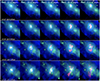 |
Fig. 1. RGB rendering of the evolution of thermal gas and passive tracers (marking relativistic electrons injected by jets) in our runs. The red colour marks the density of passive tracers, the blue the gas temperature and the green the X-ray emission. Each panel has a side of 5.5 Mpc (comoving). |
Since our runs are fully cosmological, jets swiftly interact with their surrounding environment, and they get increasingly affected and distorted by their relative motion with respect to the intracluster medium, as well a by the ram pressure of the jets’ host galaxy as it travels relative to its environment, which we measure to be v ∼ 300 km s−1. Although simulated jets were released in a perfect alignment with the z-axis of the simulation (i.e. the vertical axis in Fig. 1), their content gets dispersed also transversally to it, in a few Gyr.
At the qualitative level, the morphology of the structures that are formed by the ejected material and the mixing with the ICM resemble the appearance of observed radio lobes. However, the detectability of such features depends on the re-acceleration mechanism (see Sect. 4), and in most cases, it is only the structures formed within ≤100 Myr that are radio detectable in all models.
The various panels in Fig. 2 show the evolution of the median density, magnetic field (the one directly produced by the simulation), temperature, Mach number (only measured for shocked tracers), velocity curl (∇ × v), and velocity divergence (∇ × v) for all tracers in the various runs, as a function of time, referred to the initial epoch of jet launching, namely, z = 0.5. In the case of the magnetic field, here we show the value of the original magnetic field directly produced by our MHD simulation and the renormalised magnetic field produced based on the local solenoidal turbulence (and later used to evolve our electron spectra), as explained in Sect. 2.7.
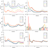 |
Fig. 2. Evolution of the median of comoving gas density, magnetic field strength, temperature, Mach number (only for shocked tracers), module of vorticity, and divergence measured by tracers in all our runs with jets. The time is measured since the start of the jets launching, i.e. from z = 0.5. In the upper right plot, we show with solid lines the trend of the original magnetic field produced by our MHD simulation, while the dotted lines display the rescaled magnetic field value, based on the local turbulent field, as estimated in Sect. 2.7. |
In order keep from introducing too much biased from the fact that, at any given time, tracers on average travel to a larger distance for runs with a larger jet power, we measured all median quantities within a radius of ≤500 kpc. In all runs, particles were subjected to the greatest fluctuations of thermodynamic values in the first ∼0.5 Gyr since their injection, which is a clear signature of the dynamics induced by jets with increasing power (which is the only different player in the different runs at this early stage). As found in Paper I, over the entire first billion years after the release of jets, the difference in the median magnetic field between runs remains always more significant than the difference in temperature. This strengthens the idea that the non-thermal content of jets delivers a long lasting memory of ancient AGN events into the ICM, while the violent mixing of gas phases, typically promoted by the AGN itself, undoes the thermal unbalances between jets and the ICM more quickly.
Since our tracer particle carry a significantly higher magnetic field in the highest power runs (a factor ∼3 − 4 higher than in the lowest power runs, corresponding to a ∼10 larger radio power), even ∼500 − 750 Myr after the jet release, also their radio properties are expected to be a good marker of the input jet power, while at their X-ray signature (e.g. cavities) are invisible after such a long period of time (e.g. De Gasperin et al. 2012; Bîrzan et al. 2012; Croston et al. 2018). This makes the radio window a potentially very powerful probe of the past activity and energetics of AGN feedback in such sources – provided that the total energetics and age of the radio lobes can be reliably estimated during such advanced evolutionary stages.
Figure 3 gives the complementary Eulerian view of of the evolving distributions of gas density, temperature, velocity dispersion (measured here after removing the bulk gas velocity on scales ≥100 kpc, with a simple high-pass filtering approach), and magnetic field strength in the innermost r ≤ 500 kpc (comoving) sphere around the cluster centre. Here, we selected here four epochs that aptly illustrate the different changes in the visible regime among the different models. In order to better highlight the (thermo-)dynamical impact of jets on the intracluster medium, in all the panels we also show the distributions from the Run 0 model, where no jets were included. Just after the jets were launched (z = 0.495), and also after ≈60 Myr (z = 0.491), we measured increasingly more prominent tails of high gas temperature, magnetic field, and velocity dispersion going from run B to run F. For reference, before the jets were activated, the gas in this region had a median gas temperature of ∼107 K, a median velocity dispersion ∼50 − 100 km s−1, and a median magnetic field strength ∼0.1 − 0.3 μG. As soon as the jets were launched, the region experienced tails of shocked hot gas (up to T ∼ 5 × 10⁸ K in the E/F runs), high magnetic fields (∼50 − 100 μG in the E/F runs), and high transonic turbulent velocities (∼5000 km s−1, in the E/F runs). While the median values of all fields remain the same, the amplitude of the tails of temperature, magnetic field strength, and velocity roughly scale with the input jet power at z = 0.491 (i.e. ∼100 Myr since the jet injection) and present a clear excess compared to the baseline (Run 0) model without jets. Based on the difference between the various velocity distributions, we can say that up to ∼100 Myr since the injection of jets, the ICM can develop a ∼10 times higher turbulent velocity compared to the baseline level induced by matter accretions in this system, for at least ∼10% of the central volume being considered here. For longer evolutionary times, the distribution of all fields in the central regions settle to very similar distributions, with the most significant exception in the distribution of magnetic fields, which remain larger even at z = 0.391 (i.e. after ≈800 Myr since the release of jets). This is consistent with our Lagrangian analysis above (see Fig. 2).
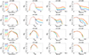 |
Fig. 3. Distributions of gas density, gas temperature, velocity dispersion, and magnetic field strength for four epochs, for a reference comoving 13 Mpc3 around the (moving) cluster center of mass at four different redshifts. For comparison, we also report the distributions from the Run 0, without jets (grey lines). |
It is only after ∼2 Gyr of evolution since the release of jets (z = 0.254 in the figure) that all distributions become similar to each other, as well as similar to the baseline (Run 0) model without jets, thus broadly marking the maximum time after which a single, powerful jet episode can leave significant dynamical difference in the host gas environment. There is one noticeable exception, however: the distribution of gas density in run E/F is significantly lowered (by a factor ∼50%), which we interpret as the integrated effect of the gas diffusion promoted by jets in these latter two runs.
In order to monitor the circulation of matter ejected by jets, we used our Lagrangian tracers and a simple metric to assess their global dispersal with time. Unlike the study Paper I, here we explored two options to compute such distance: (a) by comparing the median distance covered by tracers with respect to their initial location in the absolute reference frame of the simulation (i.e. the cells where jets were first injected) and (b) by computing the distribution of distances at every snapshots, with respect to the position of the moving galaxy, which is reasonably marked by the center of mass of the distribution of tracers. While the first choice (adopted in Paper I) is the standard approach to compute the pair dispersion statistics of Lagrangian particles in idealised turbulent simulations, the second is motivated by the fact that the center of mass of the tracer distributions, together with the galaxy hosting jets, travels across the ICM with a velocity of ∼300 km s−1. The time evolution of the mean distance of tracers, measured in these two ways, is given in Fig. 4.
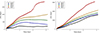 |
Fig. 4. Evolution of the median distance travelled by tracers in all runs, either with respect to the particle center of mass at all epochs (left panel), or with respect to their initial injection site (right panel). The time is measured since the start of the jets launching, i.e. from z = 0.5. |
Regardless of the approach that is adopted, tracers clearly travel on average out to a larger distance if the jet power is larger. However, there is no simple fit formula for the observed ⟨D(t)⟩ at all observed epochs. In the lowest power runs (B,C,D), the jets are not powerful enough to break out of the cluster core (≤100 kpc from the centre), which has a total thermal energy Ecore ≈ 7 × 1058 erg, and the average separation of particles relative from the SMBH settles to a constant value, with a normalisation dependent on the initial jet power. This is understandable because in the higher power runs, the initial launching phase propels a fraction of tracers to beyond the cluster core where mixing motions by cluster-wide turbulent motions become dominant (e.g. Lau et al. 2009; Angelinelli et al. 2020) and continue to spread tracers to even larger radii, in a turbulent diffusion process (Vazza et al. 2010).
While we could not find a good, simple relation that can fit the entire measured trend of the distance ⟨D(t)⟩ across the time range of our simulated outputs, a simple ⟨D(t)⟩ ∝ tw relation is found to provide a good fit for the average tracer expansion in the first ≤400 Myr after the jets’ injection, with slopes for the  relation of w = 0.082 ± 0.007 (run B), w ≈ 0.351 ± 0.021 (run C), w ≈ 0.564 ± 0.0194 (run D), w ≈ 0.653 ± 0.02 (run E), and w ≈ 0.690 ± 0.028 (run F), respectively.
Predicting the exact expansion rate of jets into the surrounding halo atmosphere is a non-trivial task (e.g. Begelman & Cioffi 1989), even in the simplistic case of static power-law density profiles, (ρ(R)∝R−α) is non-trivial, due to a number of effects related to the later expansion of jets, their progressive entrainment of the surrounding halo gas, and the onset of fluid instabilities (e.g. Bourne & Sijacki 2017). The average expansion relation measured for our tracers, at least for the most powerful runs, is approximately linear with time, unlike the softer ∝t0.7 trend reported by Perucho & Martí (2007) towards the end (∼7 Myr) of their high-resolution simulation of a Fanaroff-Riley type I source, designed to model the propagation of a P ≈ 1045 erg s−1 jet into an atmosphere resembling the real 3C31 radio galaxy. In principle, a number of important differences can account for such discrepant behaviour: unlike in previous works, the resistance of the surrounding ICM, swept up by the expanding lobes, becomes increasingly more important and, in addition, the interaction with pre-existing turbulent motions further affects the expansion dynamics of the jets, but widening the aperture of the initial velocity cone. Furthermore, from the sharp drop of temperature and density in Fig. 2, we can clearly see that the pressure in the lobes is strongly affected by expansion (and further dissipation of thermal gas energy into the environment). For all these reasons, deriving an analytical estimate of the ⟨D⟩(t) relation, also depending on the varying jet power, is non trivial (and beyond the scope of this work).
An interesting astrophysical application of our simulation is to investigate to which extend it would be possible to derive the total jet power in each model, provided that the jet injection epoch can be robustly inferred from observations (e.g. via modelling the radio emission spectra of radio lobes or from the modelling of X-ray cavities carved by jets into the hot surrounding atmosphere). Figure 5 gives the measured average distance of tracers after 100, 200, 500, and 1000 Myr since the start of jets, as function of the input jet power. At all epochs, the measured average distance is reasonably well fitted by a  relation, with the best fit parameters given in Table 2.
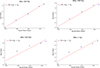 |
Fig. 5. Relation between the average distance reached by tracers in four different epochs, as a function of the input jet power in the five runs. The time is measured since the start of the jets launching, i.e. from z = 0.5. |
Best-fit parameters for the  relation between the average distance covered by tracers and the input jet power, for five different epochs.
In particular, for epochs of 100 and 200 Myr (which are also are closer to the maximum age of observable remnant radio galaxies and X-ray cavities, e.g. Wise et al. 2007; Shulevski et al. 2017) this simple fit relation can predict the overall tracer dynamics reasonably closely, meaning that for ≤200 Myr, the jet power is the main parameter determining the propagation of tracers. This suggests that the combination of an analysis of the age of particles in lobes, and of the relatively easy (at least in simple geometry cases, where projection effects can be kept under control) measurement of their average distance from their host galaxy can lead to an accurate determination of the total jet power of jets (typically with ≤5 − 10% error). In reality, the average distance covered by jets is also a function of the environment, which, in turn, is known to be strongly linked to the jet power and morphology (e.g. Hardcastle & Croston 2020, and references therein).
A systematic study of the reliability of age estimates of radio lobes based on the analysis of their observable radio spectrum will be the subject of forthcoming work (Di Federico et al., in prep.).
3.2. Spectral energy evolution of relativistic electrons
The energy evolution of electrons injected by radio galaxies is a complex combination of different mechanisms (e.g. adiabatic expansion, cooling, mixing with the ICM and re-acceleration following cluster-wide turbulence and shocks), with specific duration and features that are observed to change from run to run.
First, we focus on the evolution of the momentum spectrum for the medium power run of our suite (run D). We give, in the top row of Fig. 6, the spatial distribution of the projected number of cosmic ray electrons (computed by summing up all spectra from tracers located along the same column of 1 × 1 × 640 cells along the line of sight, each cell being 8.863 kpc3 in size) for four epochs.
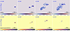 |
Fig. 6. Projected number of relativistic electrons within the same column of cells along the line of sight in run D (top), and radio emission at 50 MHz at four different epochs, in the electron model including all loss and re-acceleration terms. The blue contours in the lower raw show the regions potentially detectable with LOFAR LBA. |
The bottom row in the same figure shows instead the evolution of the radio detectable parts of the electron distribution, which we comment on later in Sect. 4. This time, the maps shows the projection along a perpendicular line of sight, as compared to Fig. 1. All re-acceleration and loss terms are considered in this case. These epochs corresponds to the emergence of very salient features in our simulated electron spectra, given in Fig. 7. In all cases (with the exception of the very first stage, in the first column) the radio detectable fraction projected volume is only a tiny fraction of the total projected volume filled by electrons, as a combined effect of adiabatic expansion and of inverse Compton and synchrotron losses, which take a few ∼102 Myr to devoid the radio-emitting part (p ≥ 104) of the momentum spectrum, for most of our simulated families of electrons. After ∼800 Myr since the jet injection (z ≤ 0.4), a steep spectrum distribution of new relativistic electrons is injected by shocks crossing the region and related to the initial AGN burst. Particles gets transported to larger distances and outside of the core, and are overall subject to the integrated effect of cooling losses (z > 0.3), which produces a classic boxy distribution in p N(p), peaking at p ∼ 103. The presence of re-acceleration by Fermi I and Fermi II mechanisms, however, makes the electron distribution to have a significantly more extended tails of particles for p ∼ 103 − 104, which, in turn, makes particle available for subsequent re-acceleration by merger-driven shocks even at later times, giving rise to a complex momentum distribution, with several bumps, as well as to a very patchy morphology of transported electron (z = 0.151). On top of this, the more continuous re-acceleration by Fermi II significantly increases the total budget of fossil electrons at p ∼ 103 − 104.
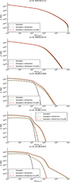 |
Fig. 7. Evolution of the momentum distributions of electrons in the run D, for five different epochs and for the three different acceleration and cooling models (colours). The dashed lines are referred to the cluster region r ≤ 300 kpc while the solid lines are for electrons at any distance from the cluster centre. |
Given the different circulation patterns of electrons, related with the jet power, which we outlined already in Sect. 3.1, we can expect increasingly different morphologies and spectral signature of the ICM dynamics when closely comparing our different runs.
The top panels of Figs. 8 and 9 again show the spatial distribution of the projected number of cosmic ray electrons, for the same epochs of Fig. 6. Clearly, already at z ≈ 0.4 the volume filling factor of electrons is larger than in the previous case, and more substructures are visible in the spatial distribution of the expanding lobes, which is understood by the increased ICM dynamics, also as a result of the shocks and turbulence injected by higher power AGN jets in run E and F. The spatial distribution of electrons injected in Runs B and C is considerably smaller (not shown, but see Fig. 1) as the bulk of electrons is confined within ≤400 kpc from the cluster centre (e.g. Sect. 3.1). Also in these cases, the radio detectable part of the electron distribution is just a tiny fraction of the underlying, undetectable and distribution of “fossil” electrons predicted by our models.
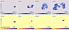 |
Fig. 8. Projected number of relativistic electrons in run E (top) and radio emission at 50 MHz at four different epochs, in the electron model including all loss and re-acceleration terms. The blue contours in the lower raw show the regions potentially detectable with LOFAR LBA. |
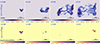 |
Fig. 9. Projected number of relativistic electrons in run F (top) and radio emission at 50 MHz at four different epochs, in the electron model including all loss and re-acceleration terms. The blue contours in the lower raw show the regions potentially detectable with LOFAR LBA. |
The reason for the quick disappearance from the radio band of such a large amount of electrons is best explained by the comparison of the particle spectra for all runs; for two of the epochs above, given in Figs. 10 and 11: at an epoch of t ∼ 800 Myr since the injection (z = 0.39, corresponding to the second row of plots in Fig. 1 and roughly marking the epoch of maximum distance from the source reached by particles in the lowest energy runs) and t ∼ 3.4 Gyr since the injection (z = 0.14, corresponding to the fourth row of plots in Fig. 1, which roughly corresponds to a high dynamical activity in the ICM, following the last major accretion episode in the host group).
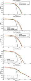 |
Fig. 10. Momentum distributions of electrons at z ≈ 0.39 in our five runs (i.e. ≈760 Myr after the jet injection), for the three different acceleration or cooling models (colours). The dashed lines are referred to the cluster region r ≤ 300 kpc while the solid line (here overlapping with the first) are for electrons at any distance from the cluster centre. The lowest power run B is at the top and the highest power run F is at the bottom. |
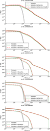 |
Fig. 11. Momentum distributions of electrons at z = 0.13 in our five runs (i.e. ≈3.2 Gyr after the jet injection), for the three different acceleration or cooling models (colours) and marking the core cluster region r ≤ 300 kpc (dashed) or the entire cluster volume (solid). The lowest power run B is at the top and the highest power run F is at the bottom. |
At both epochs (and in general), the spectra show a tendency to produce an increasingly extended tail of high energy electrons (γ ≥ 104) with the increase of the jet power. As we saw in the previous section, this stems from the combination of electrons being pushed to larger cluster radii (where they are subject to lower energy losses and to typically more efficient shock and turbulent re-acceleration) as well as to the increased ICM dynamical activity promoted by more powerful AGN, which, in turn, also enhances particle re-acceleration.
With our simulations, we can estimate the plausible budget of relativistic electrons that can be injected in the ICM by the activities of radio galaxies. To measure this, we computed the ratio between the total energy of relativistic electrons:
and the total gas energy sampled by each tracers,  , as a function of time and for the different runs. Figure 12 gives the distribution of Ecr/Eg for all tracers in the simulated volume, at the same four epochs considered above.
 |
Fig. 12. Distributions of the ratio between the total energy of all relativistic electrons we evolved in our runs at four different epochs, and the thermal gas energy associated with the same tracers. The solid lines give the distribution of Ecr/Eg for the electron evolution model including shocks and turbulent re-acceleration, while the dashed lines are for the electron model only including radiative losses and adiabatic changes after the injection by jets. |
Figure 12 gives the distribution of the energy ratio within the entire volume, for the same four epochs and runs considered above, and contrasting the prediction from the electron evolution model with shocks and turbulent re-acceleration (solid), with the model only including radiative losses and adiabatic changes (dashed). We did not divide these distributions as a function of the distance from the cluster centre as there is no significant dependence with radius (not shown). After ∼100 Myr since the jet release, the energy ratio in the lobes is Ecr/Eg ∼ 10−3, but as the mixing with the ICM proceeds, the distribution widens and stretches to smaller values. At late epochs, we observe the progressive increase of the peak distribution of Ecr/Eg as a function of the initial jet power, with values ranging from Ecr/Eg ∼ 10−5 in run B to Ecr/Eg ∼ 2 × 10⁻⁴ (with tails stretching to larger values) in run E and F. Combined with the spectral evolution presented above, these trends can be understood in the context of higher power runs, where particles are typically spread to larger cluster radii, where the role of non-thermal energy components is greater, and particles suffer fewer of synchrotron and Coulomb losses. On the other hand, the role of re-acceleration processes is not dramatic here because the Ecr/Eg ratio is dominated by the low energy part of spectra: as can seen by comparing the solid and dashed distributions of each colour in Fig. 12, Ecr/Eg does not dramatically change with the inclusion of re-acceleration terms.
Finally, we show in Fig. 13 the same distribution of energy ratios, but only limited to the p ≥ 103 part of the electron momentum distribution, which more closely tracks the budget of fossil electrons in the ICM. In this case, the role of re-acceleration terms is dominant, and at all epochs (but the very initial stage after the jet injection) and models the formation of reservoirs of fossil electrons with Ecr/Eg ≥ 10−8 is possible only when re-acceleration is present (otherwise the energy ratio is seen to be a factor ≥102 smaller).
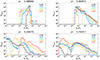 |
Fig. 13. Distributions of the ratio between the total energy of all relativistic electrons we evolved in our runs at four different epochs, and the thermal gas energy associated with the same tracers. The solid lines give the distribution of Ecr/Eg for the electron evolution model including shocks and turbulent re-acceleration, while the dashed lines are for the electron model only including radiative losses and adiabatic changes after the injection by jets. This figure only includes P/(mec)≥103 electrons in the computation of Ecr. |
4. Observable radio properties
For each tracer in the simulation, we computed its associated synchrotron radio emission for seven frequencies (50, 140, 650, 1400, 3000, 5000, and 10 000 MHz), using the formalism outlined in Sect. 2.6.
The lower rows of Figs. 6–9 show the radio synchrotron maps at 50 MHz for runs D, E, and F at four epochs (always for the model with all loss and re-acceleration terms included), which gives an idea of the structures that may (in principle) be detectable with deep LOFAR Low Band Antenna (LBA observations). To estimate the fraction of the emission that would be detectable, we considered a fixed luminosity distance of dL = 132 Mpc for all snapshots, in which case our simulated pixel size corresponds to the resolution beam of LOFAR LBA (≈8 kpc, considering a beam of θ = 12.5″), and a LOFAR LBA sensitivity of σ = 5.7 × 10⁻⁴ Jy beam−1 (here we considered ≥σ detections), which can currently be achieved with ≈72 h of integration (A. Botteon, priv. comm.).
From the figures, it can be readily seen that the emission detectable even with a deep LOFAR LBA observation is only a small fraction of the entire reservoir of electrons released by radio galaxies into the ICM. The detectable structures are often associated with weak shocks, leading to small radio relic-kind of emissions, or with the most turbulent patches of the ICM, leading to more irregular patches of emission, even on scales that are apparently not filled by non-thermal plasma associated with visible radio lobes.
The integrated radio spectra, after the initial injection phase, are generally very steep, owing to the depletion of electrons with γ ≥ 5 × 10³, which are mostly responsible for the emission at ν ≥ 50 MHz. The radio spectra for the evolving run D are shown in Fig. 14, while the comparison between the five runs at two different epochs (the same of Figs. 10 and 11) are shown in Fig. 15.
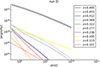 |
Fig. 14. Evolution of the synchrotron radio spectra of all electrons in the run D, for ten different epochs. The solid lines are the spectra including all loss and re-acceleration terms, the dashed line are for models including all loss terms and shock (re)acceleration, while the dotted lines are for models that include only loss terms. |
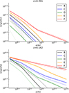 |
Fig. 15. Synchrotron radio spectra in our five runs at z = 391 (i.e. ≈760 Myr after the jet injection) and at z = 0.142 (≈3.2 Gyr after the jet injection). The solid lines are the spectra including all loss and re-acceleration terms, the dashed line are for models including all loss terms and shock (re)acceleration, while the dotted lines are for models including only loss terms. |
The distribution of radio spectral indices between 50 and 140 MHz, for ≥σ detectable pixels, is shown in Fig. 16 for four different epochs in run E, showing the predictions for the three electron evolution scenarios: after z ≥ 0.48, the only detectable patches are clearly related with the turbulent re-acceleration model, leading even to extremely steep (α ≥ 2 − 3) and small structures. The only contribution of shock re-acceleration can produce fewer detectable pixels, typically with 1 ≤ α ≤ 2 depending on the shock Mach number. No emission can be detected after ≈200 Myr if the energy of relativistic electrons injected by radio galaxies solely evolves under radiative losses and adiabatic changes.
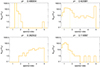 |
Fig. 16. Distributions of radio spectral index between 140 and 50 MHz, only for ≥1σrms detectable pixels in radio maps of the run E at four different epochs. The solid lines give the distribution of distribution of spectra for the electron evolution model including shocks and turbulent re-acceleration, the dashed lines are for the electron model only including shock re-acceleration and loss terms, and the dotted lines are for the electron model only including radiative losses and adiabatic changes after the injection by jets. |
We shall remark that our assumed ≥σ detection criterion is optimistic and is meant to highlight the tip of the iceberg of the potentially detectable structures in radio. State-of-the-art imaging pipelines typically detect diffuse emission from ≥2σ at most (e.g. Botteon et al. 2018). However, our recent works have shown that new signal analysis strategies based on machine learning (Gheller et al. 2018) or convolutional deep denoising autoencoders (Gheller & Vazza 2022) can potentially detect diffuse correlated emission even at the ∼0.1σ level, when opportunely trained with large training sets and under ideal observing conditions. While it is still a challenge to quantitatively estimate the actual gain in detection level compared to more standard techniques under realistic noise condition, such techniques are being broadly explored as a solution to the challenges that the Square Kilometer Array (SKA) will pose to the community (e.g. Yu et al. 2022), including the detection and classification of the flurry of data from radio galaxies that future surveys will deliver (e.g. Becker et al. 2021; Tang et al. 2022, for recent works on this topic). All this considered, the adopted ≥σ detection criterion considered here is a reasonable intermediate estimate between what is currently possible and what should soon be achieved by standard detection algorithms to exploit the vastness of modern radio surveys.
For all runs, the distributions of detectable spectral indices, measured at the same epochs, confirm these trends: Figure 17 shows that at most epochs the detectable emission is dominated by steep spectra and, generally, runs with a higher power lead to a larger number of detectable and steep emission patches.
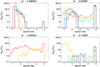 |
Fig. 17. Distributions of radio spectral index between 140 and 50 MHz, only for ≥1σrms detectable pixels in radio maps of all runs at four different epochs, only for the electron evolution model including all loss and re-acceleration terms. |
The detection of such steep spectra emission is challenging and calls for sensitive low-frequency radio observations. However, the detection of such structures has become increasingly more common with LOFAR and MWA, as well as several extremely steep spectrum sources that are often associated with remnant plasma from radio galaxy activity and possibly interacting with the ICM, which have been reported in the latest years: De Gasperin et al. (2017; α = 4.5 in Abell 1033), Biava et al. (2021b; α = 3.2 in RX J1720.1+2638), Hodgson et al. (2021; α = 5.97 in Abell 2877). In particular, some of the simulations analysed in Paper I were indeed already used by Hodgson et al. (2021) for the interpretation of real MWA data. They argued that the late evolution of fossil radio plasma – which can produce short-distance (≤100 Myr) detectable structures where a few remnant lobes mix and get compressed by weak shocks triggered by ICM activity – can represent a viable scenario for the formation of such diffuse steep-spectrum sources.
Recent works have investigated the relation between the radio power of central radio galaxies and the X-ray luminosity of the host cluster (Pasini et al. 2020). In particular, Pasini et al. (2022) observed 227 radiogalaxies with LOFAR-HBA (140 MHz) and correlated their radio emission with the X-ray emission in the 0.5−2 keV band, in the eROSITA Final Equatorial Depths Survey (eFEDS), reporting a positive correlation between the two quantities, as well as large scatter in radio power for any given X-ray luminosity.
We can produce a similar statistics in our runs by computing the total radio emission from our electrons at 140 MHz, compared to the X-ray emission computed from the simulated gas distribution, in which we assumed a single temperature value for each simulated cell, a constant composition (with metallicity Z/Z⊙ = 0.3), and collisional equilibrium. This allowed us to use the emissivity, Λ, from the B-Astrophysical Plasma Emission Code (B-APEC)4, and to compute the total X-ray (continuum and line) emission within the same eROSITA energy band.
This is shown in Fig. 18, where we plot the evolution of the total radio emission from our electrons (in the two extreme cases where only injection and cooling are considered or when all re-acceleration processes are also used), within the same fixed area (≤500 kpc) from the group centre used by Pasini et al. (2022).
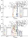 |
Fig. 18. Evolution of the total radio emission within ≤500 kpc from the group centre at 140 MHz, as a function of the X-ray emission in the [0.5−2] keV range within the same region, from z = 0.5 to z = 0.4 and for our five runs. The top panel shows our prediction for a model in which electrons are injected by jets and are then only subject to radiative and adibatic changes, while in the lower panel all re-acceleration mechanisms are considered. The grey points show the real LOFAR-HBA and eRosita observations from Pasini et al. (2022). |
While it is impossible with our single simulated group to establish of a correlation between X-ray and radio power, we can study the impact of the jet power in the simulated X-ray and radio emission as a function of time. In the simulated case, the X-ray luminosity is little affected by the jet bursts (the X-ray luminosity from the innermost region only varies by a factor of ∼2 at most in the time interval under consideration) but the radio emission changes by many orders of magnitude in the same period of time. If we compare the same absolute epoch, the relative drop of the radio emission is much less pronounced for a higher jet power: for example, at the reference epoch of z = 0.4 (as shown in the plots), the radio emission in run F has dropped by a factor of ∼103 compared to the initial value, while this is ∼4 × 10⁴ in run E and this is ≥106 in the lowest power runs (albeit with in a non-monotonic way, due to re-acceleration mechanisms). If no-reacceleration mechanism is considered, all simulated evolution show a quick crossing of the range spanned by real observations, followed by a longer stage of undetectable radio emission. On the other hand, when Fermi I and Fermi II re-acceleration are allowed, the radio emission drops more slowly with time, and at least in the two highest power runs the remnant radio emission remain for a longer period of time within the range of real observations.
Interestingly, we find that our jets have a different impact on the X-ray emission of the group, namely, depending on their initial power, the total X-ray luminosity of the group is found to alternatively increase (in low power jets) or decrease (in the highest power cases) over time, with the medium power run (D, Pj = 3 × 1044 erg s−1) roughly separating the two regimes. Jets with Pj ≥ 9 × 1043 erg s−1 (run E and D) are powerful enough to smooth the gas core density, carve prominent X-ray cavities and reduce (by a factor ∼50%) the core X-ray emission until z = 0.4.
Conversely, jets with Pj ≤ 1044 erg s−1 reduce the X-ray emission from the core only in the very first stage of activity, while later on the group increases its X-ray emission owing to the gradual increase in its density, due to the effect of subsequent matter accretions, and of the related crossing of new substructures in the cluster atmosphere. The above trends makes run E and F able to produce two overall positively correlated trajectories in the (L140, LX) plane, as in observations, while the other produce a negative and steep correlation between radio and X-ray powers, for the time in which (some) of their the radio emission is detectable.
Although it is impossible to reliably use these trends to compare to the observed positive correlation reported by Pasini et al. (2020), it is interesting to notice that the large amount of vertical evolution in all our runs does not seem in conflict with the large scatter in real observations, even in the very homogeneous selection presented by Pasini et al. (2022). This suggests that the observed scatter might not be caused by the host cluster, but rather that it may trace the complex evolution of real sources through the (L140, LX) plane on a time scale that depends on the power of the underlying radio jet.
5. Discussion: Ways jet power influences the evolution of radio emission
Our simulations helped us to identify several relations between the input jet power (of a single episode of AGN feedback) and the late-time (≥100 Myr) evolution of injected relativistic particles and of their associated radio signal. First, we know that the magnetisation of jets (followed by the magnetisation of remnant lobes) depends on the input jet power for ∼1 Gyr since the jet release (Figs. 2 and 3).
Depending on the initial power of jets, the injected particles can exit the cluster core and continue to be dispersed up to the cluster virial radius by large-scale turbulent motion, or, instead, remain confined around the cluster core (Fig. A.1). For the M100 ≈ 2 × 10¹⁴ M⊙ host system considered in this work, the critical jet power appears to be in the Pj ≥ 3 − 9 × 1044 erg s−1 range.
Then, the typical distance reached by electrons at fixed times is a regular function of the jet power (Fig. 5), which can be well described by a  dependence up to ∼1 − 2 Gyr since the injection of jets. In addition, the budget of relativistic electrons a few Gyr after the injection is found to increased with Pj (Figs. 12 and 13), albeit typically with a complex relation that depends on the time-integrated effects of energy losses and re-acceleration terms.
Consequently, the radio emission at a given frequency is also typically higher at any given time for higher jet powers, even if in this case spectral effects at different frequencies further complicate the search for simple trends. In general, we find that the stronger the initial jet power, the longer do radio lobes remain inside the range of typical radio luminosities, always with very steep radio spectra (Figs. 17 and 18).
Our conclusions are based on a single and impulsive (≤32 Myr) AGN burst for each resimulation. It is only thanks to more sophisticated simulations that we will be able to assess the amplitude of such differences in the presence of multiple AGN feedback events and with bursts of different durations.
6. Caveats and discussion
In this section, we briefly comment what we believe are the most important weaknesses and the range of validity of the theoretical work presented here.
First, our simulations are uniquely concerned with the single fluid ideal MHD approach, namely, resistive and multi-fluid effects are entirely neglected. Therefore, since the viscous and resistive scales are essentially the same, our simulations refer to an ICM which has a magnetic Prandtl number PM = ν/η ≈ 1 (where ν is the kinematic viscosity and η is the resistivity), which surely is an unrealistic assumption (e.g. Schekochihin et al. 2004; Brunetti & Lazarian 2011; Beresnyak & Miniati 2016). To probe the small-scale dynamo, the entirely different and computationally expensive type of kinetic simulations are needed (e.g. Rincon et al. 2016). In this work, we are not concerned with the effects of dynamo amplification, which is bound to be underestimated at this resolution anyway. To bracket the likely value of magnetic field amplification produced by plasma processes below our resolution scale, we used the post-processing recalibration of the magnetic field on tracers (Sect. 2.7).
Another important limitation of this suite of simulation is that, for the sake of simplicity, we did not even attempt to self-consistently link the cooling-heating cycle of baryons induced by AGN feedback, which would introduce a number of numerical and physical complications which are far from being solved in cosmological simulations (e.g. Negri & Volonteri 2017; Habouzit et al. 2022, and references therein).
Having established with this first work (jointly with Paper I) the role between jet energetics and the circulation of non-thermal electrons, we defer to future work to design efficient numerical modules in ENZO also to couple jets to the mass growth of SMBH, with a further distinction between hot and cold gas accretion modalities (e.g. Thomas et al. 2021).
Moreover, our treatment of jets is not suitable to follow the actual interaction between the relativistic (either electron- or proton-dominated) content of jets and the thermal ICM. Our jets are entirely made of hot gas and magnetic fields. This choice is very commonly adopted in the literature, and is not expected to significantly affect the long-term (≥100 Myr) evolution of the jets, or of the particles they carry. However, on small evolutionary stages the effective equation of state of a truly cosmic-ray dominated jet may produce somewhat different dynamics (Ehlert et al. 2018), also related the very first, relativistic bulk motion of jets (Perucho et al. 2017).
In summary, the simulated large-scale (≥100 kpc) and long-term (≥100 Myr) circulation of our jets and of the injected lobe remnants is reasonably well captured by our model. Yet the small-scale interplay between gas, magnetic fields and cosmic rays, as well as the coupling with the mass growth process of SMBH deserve more extended, ad hoc simulations.
7. Conclusions
We present new simulations of the evolution of relativistic electrons injected by radio galaxies in the ICM, studying how the spatial and energy evolution of electrons is changed by the increase of the jet power. We modelled the evolution of electrons based on the assumptino that they are ‘passively’ advected by flows in the ICM and we studied the evolution of their energy spectra by including realistic loss and gain terms. Our main results can be summarized as follows:
-
The propagation of tracers in the ICM is the combination of an initial stage (≤200 Myr since the release of jets) mostly dominated by jet dynamics, followed by a longer (≥2 Gyr since the release of jets) second stage that is dominated by the diffusion by ICM turbulent motions. The final average distance covered by electrons, at fixed epochs, is found to strongly depend on the input jet power, through a well-constrained
 relation.
 -
Our simulated jets do not cause significant thermodynamical differences in the evolution of the ICM that can be detected after about ∼500 Myr since their burst. On the other hand, magnetic fields in the ICM are affected by jets even ∼1 Gyr after the burst.
-
Depending on the input jet power and on the efficiency of Fermi I and Fermi II re-acceleration on the injected electrons, the innermost ICM volume can have a cosmic ray (electron) to thermal gas energy ratio in the range ∼10−6 to ∼10−4 even ∼3 Gyr since the jet release (with the latter being produced by higher power jets, and with efficient Fermi II re-acceleration from the ICM). This budget comes from the vast majority of fossil γ ≤ 103 electrons, originally injected by the single central radio galaxy simulated in this works, Hence, this constitutes a lower limit on the real electron budget in the ICM.
-
The spectrum of radio-emitting electrons, already after ∼200 Myr since the jet injection, crucially depends on the ICM dynamics capable of re-accelerating fossil electrons injected by radio galaxies. Only if Fermi I and Fermi II processes are considered, the remnant electrons can become detectable again later in the cluster evolution, typically at low frequencies and with very steep radio spectra (α ≥ 2).
This work confirms that the ICM can be enriched at low redshifts with a volume-filling population of fossil relativistic electrons, seeded by radio galaxies. The ICM dynamics induced by mergers can re-energise this population leading to diffuse radio emission (e.g. Sarazin 1999; Brunetti & Jones 2014; Van Weeren et al. 2019).
While the existence of such a reservoir of fossil electrons is a mere hypothesis, and the question of whether or not radio galaxies could produce them in their lifetime remains unproven, our simulations supports that this mechanism is realistic, for a range of jet powers and coupling between ICM dynamics and particle re-acceleration.
Recent low-frequency observations of nearby radio sources in clusters and groups of galaxies have started scratching the surface of the low-frequency emission from remnant electrons (e.g. De Gasperin et al. 2017; Wilber et al. 2018; Mandal et al. 2020; Hodgson et al. 2021; Brienza et al. 2021, 2022) and new numerical simulations of these complex processes represent a tool to constrain non-thermal physics in clusters. The issues of whether the single release of relativistic electrons by a radiogalaxy in the ICM is enough to contribute all fossil relativistic electron required to reproduce the morphology and observed power of most radio relics or radio halos or (instead) whether multiple radio galaxies and a more extended activity period is required will be subject of follow-up investigations.
Moreover, the evidence that already for ≥100 Myr, the distribution of the spectral index in lobes mixing with the ICM has different shapes depending on the underlying re-acceleration mechanisms suggests that, in general, age estimates based on the modelling of radio spectra would increasingly overestimate the age of sources, if only loss and adiabatic terms are included in the modelling (see also Paper I). A further analysis of this aspect will be the subject of future work.
We share the public version of our ROGER solver at the url https://github.com/FrancoVazza/JULIA/tree/master/ROGER
We notice that our group has also recently explored more self-consistent dependencies between the minimum momentum of electrons and the shock acceleration efficiency (Inchingolo et al. 2022), following Kang (2021), yet here we prefer to keep the same formalism of Paper I, for the sake of comparison.
Acknowledgments
We thank our anonymous reviewer for their very detailed and helpful comments to the first version of this draft. The authors gratefully acknowledge the Gauss Centre for Supercomputing e.V. (https://www.gauss-centre.eu) for supporting this project by providing computing time through the John von Neumann Institute for Computing (NIC) on the GCS Supercomputer JUWELS at Jülich Supercomputing Centre (JSC), under projects ‘radgalicm’ and ‘radgalicm2’. F.V. acknowledges financial support from the European Union’s Horizon 2020 program under the ERC Starting Grant ‘MAGCOW’, no. 714196. D.W. is funded by the Deutsche Forschungsgemeinschaft (DFG, German Research Foundation) – 441694982. M.B. acknowledges support from the Deutsche Forschungsgemeinschaft under Germany’s Excellence Strategy – EXC 2121 “Quantum Universe” – 390833306. T.P. is supported by the DLR Verbundforschung under grant number 50OR1906. Finally, we made use of the Cosmological Calculator by E. Wright (https://www.astro.ucla.edu/~wright/CosmoCalc.html).
References
- Angelinelli, M., Vazza, F., Giocoli, C., et al. 2020, MNRAS, 495, 864 [NASA ADS] [CrossRef] [Google Scholar]
- Banfi, S., Vazza, F., & Wittor, D. 2020, MNRAS, 496, 3648 [NASA ADS] [CrossRef] [Google Scholar]
- Becker, B., Vaccari, M., Prescott, M., & Grobler, T. 2021, MNRAS, 503, 1828 [NASA ADS] [CrossRef] [Google Scholar]
- Begelman, M. C., & Cioffi, D. F. 1989, ApJ, 345, L21 [CrossRef] [Google Scholar]
- Beresnyak, A., & Miniati, F. 2016, ApJ, 817, 127 [NASA ADS] [CrossRef] [Google Scholar]
- Biava, N., Brienza, M., Bonafede, A., et al. 2021a, A&A, 650, A170 [NASA ADS] [CrossRef] [EDP Sciences] [Google Scholar]
- Biava, N., de Gasperin, F., Bonafede, A., et al. 2021b, MNRAS, 508, 3995 [NASA ADS] [CrossRef] [Google Scholar]
- Bîrzan, L., Rafferty, D. A., McNamara, B. R., Wise, M. W., & Nulsen, P. E. J. 2004, ApJ, 607, 800 [Google Scholar]
- Bîrzan, L., Rafferty, D. A., Nulsen, P. E. J., et al. 2012, MNRAS, 427, 3468 [Google Scholar]
- Booth, C. M., & Schaye, J. 2009, MNRAS, 398, 53 [Google Scholar]
- Botteon, A., Shimwell, T. W., Bonafede, A., et al. 2018, MNRAS, 478, 885 [Google Scholar]
- Botteon, A., Brunetti, G., van Weeren, R. J., et al. 2020a, ApJ, 897, 93 [Google Scholar]
- Botteon, A., Brunetti, G., Ryu, D., & Roh, S. 2020b, A&A, 634, A64 [NASA ADS] [CrossRef] [EDP Sciences] [Google Scholar]
- Bourne, M. A., & Sijacki, D. 2017, MNRAS, 472, 4707 [NASA ADS] [CrossRef] [Google Scholar]
- Brienza, M., Godfrey, L., Morganti, R., et al. 2016, A&A, 585, A29 [NASA ADS] [CrossRef] [EDP Sciences] [Google Scholar]
- Brienza, M., Morganti, R., Harwood, J., et al. 2020, A&A, 638, A29 [EDP Sciences] [Google Scholar]
- Brienza, M., Shimwell, T. W., de Gasperin, F., et al. 2021, Nat. Astron., 5, 1261 [NASA ADS] [CrossRef] [Google Scholar]
- Brienza, M., Lovisari, L., Rajpurohit, K., et al. 2022, A&A, 661, A92 [NASA ADS] [CrossRef] [EDP Sciences] [Google Scholar]
- Brunetti, G., & Jones, T. W. 2014, Int. J. Mod. Phys. D, 23, 1430007 [Google Scholar]
- Brunetti, G., & Lazarian, A. 2010, MNRAS, 378, 245 [Google Scholar]
- Brunetti, G., & Lazarian, A. 2011, MNRAS, 410, 127 [Google Scholar]
- Brunetti, G., & Lazarian, A. 2016, MNRAS, 458, 2584 [Google Scholar]
- Brunetti, G., & Vazza, F. 2020, Phys. Rev. Lett., 124, 051101 [Google Scholar]
- Bryan, G. L., Norman, M. L., O’Shea, B. W., et al. 2014, ApJS, 211, 19 [Google Scholar]
- Candelaresi, S., & Del Sordo, F. 2020, ApJ, 896, 86 [CrossRef] [Google Scholar]
- Chang, J. S., & Cooper, G. 1970, J. Comput. Phys., 6, 1 [Google Scholar]
- Chatterjee, K., Markoff, S., Neilsen, J., et al. 2021, MNRAS, 507, 5281 [NASA ADS] [CrossRef] [Google Scholar]
- Chibueze, J. O., Sakemi, H., Ohmura, T., et al. 2021, Nature, 593, 47 [NASA ADS] [CrossRef] [Google Scholar]
- Croston, J. H., Hardcastle, M. J., Birkinshaw, M., Worrall, D. M., & Laing, R. A. 2008, MNRAS, 386, 1709 [NASA ADS] [CrossRef] [Google Scholar]
- Croston, J. H., Ineson, J., & Hardcastle, M. J. 2018, MNRAS, 476, 1614 [Google Scholar]
- Dedner, A., Kemm, F., Kröner, D., et al. 2002, J. Comput. Phys., 175, 645 [Google Scholar]
- De Gasperin, F., Orrú, E., Murgia, M., et al. 2012, A&A, 547, A56 [NASA ADS] [CrossRef] [EDP Sciences] [Google Scholar]
- De Gasperin, F., Intema, H. T., Shimwell, T. W., et al. 2017, Sci. Adv., 3, e1701634 [NASA ADS] [CrossRef] [Google Scholar]
- Ehlert, K., Weinberger, R., Pfrommer, C., Pakmor, R., & Springel, V. 2018, MNRAS, 481, 2878 [NASA ADS] [CrossRef] [Google Scholar]
- Fabian, A. C. 2012, ARA&A, 50, 455 [Google Scholar]
- Fabjan, D., Borgani, S., Tornatore, L., et al. 2010, MNRAS, 401, 1670 [Google Scholar]
- Fouka, M., & Ouichaoui, S. 2014, MNRAS, 442, 979 [NASA ADS] [CrossRef] [Google Scholar]
- Gaspari, M., & Churazov, E. 2013, A&A, 559, A78 [NASA ADS] [CrossRef] [EDP Sciences] [Google Scholar]
- Gaspari, M., Brighenti, F., D’Ercole, A., & Melioli, C. 2011, MNRAS, 415, 1549 [NASA ADS] [CrossRef] [Google Scholar]
- Gaspari, M., Ruszkowski, M., & Sharma, P. 2012, ApJ, 746, 94 [Google Scholar]
- Gheller, C., & Vazza, F. 2022, MNRAS, 509, 990 [Google Scholar]
- Gheller, C., Vazza, F., & Bonafede, A. 2018, MNRAS, 480, 3749 [NASA ADS] [CrossRef] [Google Scholar]
- Godfrey, L. E. H., & Shabala, S. S. 2013, ApJ, 767, 12 [NASA ADS] [CrossRef] [Google Scholar]
- Guidetti, D., Laing, R. A., Croston, J. H., Bridle, A. H., & Parma, P. 2012, MNRAS, 423, 1335 [NASA ADS] [CrossRef] [Google Scholar]
- Guo, X., Sironi, L., & Narayan, R. 2014a, ApJ, 794, 153 [NASA ADS] [CrossRef] [Google Scholar]
- Guo, X., Sironi, L., & Narayan, R. 2014b, ApJ, 797, 47 [NASA ADS] [CrossRef] [Google Scholar]
- Habouzit, M., Onoue, M., Bañados, E., et al. 2022, MNRAS, 511, 3751 [NASA ADS] [CrossRef] [Google Scholar]
- Hardcastle, M. J., & Croston, J. H. 2020, New Astron. Rev., 88, 101539 [Google Scholar]
- Hardcastle, M. J., & Krause, M. G. H. 2014, MNRAS, 443, 1482 [NASA ADS] [CrossRef] [Google Scholar]
- Harwood, J. J., Hardcastle, M. J., & Croston, J. H. 2015, MNRAS, 454, 3403 [NASA ADS] [CrossRef] [Google Scholar]
- Hodgson, T., Bartalucci, I., Johnston-Hollitt, M., et al. 2021, ApJ, 909, 198 [CrossRef] [Google Scholar]
- Inchingolo, G., Wittor, D., Rajpurohit, K., & Vazza, F. 2022, MNRAS, 509, 1160 [Google Scholar]
- Jones, T. W., Nolting, C., O’Neill, B. J., & Mendygral, P. J. 2017, Phys. Plasmas, 24, 041402 [NASA ADS] [CrossRef] [Google Scholar]
- Kang, H. 2021, J. Korean Astron. Soc., 54, 103 [NASA ADS] [Google Scholar]
- Kang, H., & Jones, T. W. 2007, Astropart. Phys., 28, 232 [NASA ADS] [CrossRef] [Google Scholar]
- Kang, H., & Ryu, D. 2011, ApJ, 734, 18 [Google Scholar]
- Kang, H., Ryu, D., & Jones, T. W. 2012, ApJ, 756, 97 [Google Scholar]
- Kim, J.-H., Wise, J. H., Alvarez, M. A., & Abel, T. 2011, ApJ, 738, 54 [NASA ADS] [CrossRef] [Google Scholar]
- Komissarov, S. S., & Gubanov, A. G. 1994, A&A, 285, 27 [NASA ADS] [Google Scholar]
- Kukreti, P., Morganti, R., Shimwell, T. W., et al. 2022, A&A, 658, A6 [NASA ADS] [CrossRef] [EDP Sciences] [Google Scholar]
- Lau, E. T., Kravtsov, A. V., & Nagai, D. 2009, ApJ, 705, 1129 [NASA ADS] [CrossRef] [Google Scholar]
- Li, H., Lapenta, G., Finn, J. M., Li, S., & Colgate, S. A. 2006, ApJ, 643, 92 [NASA ADS] [CrossRef] [Google Scholar]
- Mandal, S., Intema, H. T., van Weeren, R. J., et al. 2020, A&A, 634, A4 [NASA ADS] [CrossRef] [EDP Sciences] [Google Scholar]
- Markevitch, M., Govoni, F., Brunetti, G., & Jerius, D. 2005, ApJ, 627, 733 [Google Scholar]
- Massaglia, S., Bodo, G., Rossi, P., Capetti, S., & Mignone, A. 2016, A&A, 596, A12 [NASA ADS] [CrossRef] [EDP Sciences] [Google Scholar]
- McNamara, B. R., & Nulsen, P. E. J. 2007, ARA&A, 45, 117 [NASA ADS] [CrossRef] [Google Scholar]
- Mendygral, P. J., Jones, T. W., & Dolag, K. 2012, ApJ, 750, 166 [NASA ADS] [CrossRef] [Google Scholar]
- Miley, G., & De Breuck, C. 2008, A&A Rev, 15, 67 [NASA ADS] [CrossRef] [Google Scholar]
- Mingo, B., Croston, J. H., Hardcastle, M. J., et al. 2019, MNRAS, 488, 2701 [NASA ADS] [CrossRef] [Google Scholar]
- Mingo, B., Croston, J. H., Best, P. N., et al. 2022, MNRAS, 511, 3250 [NASA ADS] [CrossRef] [Google Scholar]
- Mukherjee, D., Bodo, G., Rossi, P., Mignone, A., & Vaidya, B. 2021, MNRAS, 505, 2267 [NASA ADS] [CrossRef] [Google Scholar]
- Murgia, M., Parma, P., Mack, K. H., et al. 2011, A&A, 526, A148 [NASA ADS] [CrossRef] [EDP Sciences] [Google Scholar]
- Negri, A., & Volonteri, M. 2017, MNRAS, 467, 3475 [NASA ADS] [CrossRef] [Google Scholar]
- Nolting, C., Jones, T. W., O’Neill, B. J., & Mendygral, P. J. 2019, ApJ, 876, 154 [NASA ADS] [CrossRef] [Google Scholar]
- O’Sullivan, S. P., Brüggen, M., Vazza, F., et al. 2020, MNRAS, 495, 2607 [Google Scholar]
- Pasini, T., Brüggen, M., de Gasperin, F., et al. 2020, MNRAS, 497, 2163 [NASA ADS] [CrossRef] [Google Scholar]
- Pasini, T., Brüggen, M., Hoang, D. N., et al. 2022, A&A, 661, A13 [NASA ADS] [CrossRef] [EDP Sciences] [Google Scholar]
- Perucho, M., & Martí, J. M. 2007, MNRAS, 382, 526 [NASA ADS] [CrossRef] [Google Scholar]
- Perucho, M., Martí, J.-M., Quilis, V., & Borja-Lloret, M. 2017, MNRAS, 471, L120 [NASA ADS] [CrossRef] [Google Scholar]
- Pinzke, A., Oh, S. P., & Pfrommer, C. 2013, MNRAS, 435, 1061 [Google Scholar]
- Planck Collaboration XIII. 2016, A&A, 594, A13 [NASA ADS] [CrossRef] [EDP Sciences] [Google Scholar]
- Puchwein, E., Sijacki, D., & Springel, V. 2008, ApJ, 687, L53 [NASA ADS] [CrossRef] [Google Scholar]
- Randriamanakoto, Z., Ishwara-Chandra, C. H., & Taylor, A. R. 2020, MNRAS, 496, 3381 [NASA ADS] [CrossRef] [Google Scholar]
- Rasia, E., Borgani, S., Murante, G., et al. 2015, ApJ, 813, L17 [Google Scholar]
- Ricarte, A., Tremmel, M., Natarajan, P., & Quinn, T. 2019, MNRAS, 489, 802 [NASA ADS] [CrossRef] [Google Scholar]
- Rincon, F., Califano, F., Schekochihin, A. A., & Valentini, F. 2016, Proc. Natl. Acad. Sci., 113, 3950 [NASA ADS] [CrossRef] [Google Scholar]
- Riquelme, M. A., & Spitkovsky, A. 2011, ApJ, 733, 63 [NASA ADS] [CrossRef] [Google Scholar]
- Sarazin, C. L. 1999, ApJ, 520, 529 [Google Scholar]
- Schekochihin, A. A., Cowley, S. C., Taylor, S. F., Maron, J. L., & McWilliams, J. C. 2004, ApJ, 612, 276 [NASA ADS] [CrossRef] [Google Scholar]
- Shi, X., Nagai, D., & Lau, E. T. 2018, MNRAS, 481, 1075 [NASA ADS] [CrossRef] [Google Scholar]
- Shulevski, A., Morganti, R., Harwood, J. J., et al. 2017, A&A, 600, A65 [NASA ADS] [CrossRef] [EDP Sciences] [Google Scholar]
- Simonte, M., Vazza, F., Brighenti, F., et al. 2022, A&A, 658, A149 [NASA ADS] [CrossRef] [EDP Sciences] [Google Scholar]
- Talbot, R. Y., Bourne, M. A., & Sijacki, D. 2021, MNRAS, 504, 3619 [NASA ADS] [CrossRef] [Google Scholar]
- Tang, H., Scaife, A. M. M., Wong, O. I., & Shabala, S. S. 2022, MNRAS, 510, 4504 [NASA ADS] [CrossRef] [Google Scholar]
- Thomas, N., Davé, R., Jarvis, M. J., & Anglés-Alcázar, D. 2021, MNRAS, 503, 3492 [NASA ADS] [CrossRef] [Google Scholar]
- Tremblay, G. R., Oonk, J. B. R., Combes, F., et al. 2016, Nature, 534, 218 [NASA ADS] [CrossRef] [Google Scholar]
- Tremmel, M., Karcher, M., Governato, F., et al. 2017, MNRAS, 470, 1121 [NASA ADS] [CrossRef] [Google Scholar]
- Valdarnini, R. 2019, ApJ, 874, 42 [NASA ADS] [CrossRef] [Google Scholar]
- Vallés-Pérez, D., Planelles, S., & Quilis, V. 2021, MNRAS, 504, 510 [CrossRef] [Google Scholar]
- Van Weeren, R. J., de Gasperin, F., Akamatsu, H., et al. 2019, Space Sci. Rev., 215, 16 [NASA ADS] [CrossRef] [Google Scholar]
- Vardoulaki, E., Jiménez Andrade, E. F., Karim, A., et al. 2019, A&A, 627, A142 [NASA ADS] [CrossRef] [EDP Sciences] [Google Scholar]
- Vardoulaki, E., Vazza, F., Jiménez-Andrade, E. F., et al. 2021, Galaxies, 9, 93 [NASA ADS] [CrossRef] [Google Scholar]
- Vazza, F., Brunetti, G., Kritsuk, A., et al. 2009, A&A, 504, 33 [NASA ADS] [CrossRef] [EDP Sciences] [Google Scholar]
- Vazza, F., Gheller, C., & Brunetti, G. 2010, A&A, 513, A32 [NASA ADS] [CrossRef] [EDP Sciences] [Google Scholar]
- Vazza, F., Brunetti, G., Gheller, C., Brunino, R., & Brüggen, M. 2011, A&A, 529, A17 [NASA ADS] [CrossRef] [EDP Sciences] [Google Scholar]
- Vazza, F., Brüggen, M., & Gheller, C. 2013, MNRAS, 428, 2366 [NASA ADS] [CrossRef] [Google Scholar]
- Vazza, F., Brueggen, M., Gheller, C., et al. 2017a, Class. Quant. Grav., 34, 234001 [NASA ADS] [CrossRef] [Google Scholar]
- Vazza, F., Jones, T. W., Brüggen, M., et al. 2017b, MNRAS, 464, 210 [Google Scholar]
- Vazza, F., Brunetti, G., Brüggen, M., & Bonafede, A. 2018, MNRAS, 474, 1672 [NASA ADS] [CrossRef] [Google Scholar]
- Vazza, F., Locatelli, N., Rajpurohit, K., et al. 2021a, Galaxies, 9, 109 [NASA ADS] [CrossRef] [Google Scholar]
- Vazza, F., Wittor, D., Brunetti, G., & Brüggen, M. 2021b, A&A, 653, A23 (Paper I) [NASA ADS] [CrossRef] [EDP Sciences] [Google Scholar]
- Vernstrom, T., Heald, G., Vazza, F., et al. 2021, MNRAS, 505, 4178 [NASA ADS] [CrossRef] [Google Scholar]
- Völk, H. J., & Atoyan, A. M. 2000, ApJ, 541, 88 [CrossRef] [Google Scholar]
- Wang, P., & Abel, T. 2009, ApJ, 696, 96 [NASA ADS] [CrossRef] [Google Scholar]
- Weinberger, R., Ehlert, K., Pfrommer, C., Pakmor, R., & Springel, V. 2017, MNRAS, 470, 4530 [CrossRef] [Google Scholar]
- Wilber, A., Brüggen, M., Bonafede, A., et al. 2018, MNRAS, 473, 3536 [Google Scholar]
- Wise, M. W., McNamara, B. R., Nulsen, P. E. J., Houck, J. C., & David, L. P. 2007, ApJ, 659, 1153 [NASA ADS] [CrossRef] [Google Scholar]
- Wittor, D., Vazza, F., & Brüggen, M. 2016, Galaxies, 4, 71 [NASA ADS] [CrossRef] [Google Scholar]
- Wittor, D., Jones, T., Vazza, F., & Brüggen, M. 2017, MNRAS, 471, 3212 [NASA ADS] [CrossRef] [Google Scholar]
- Wittor, D., Vazza, F., Ryu, D., & Kang, H. 2020, MNRAS, 495, L112 [NASA ADS] [CrossRef] [Google Scholar]
- Xu, H., Li, H., Collins, D. C., Li, S., & Norman, M. L. 2009, ApJ, 698, L14 [NASA ADS] [CrossRef] [Google Scholar]
- Xu, R., Spitkovsky, A., & Caprioli, D. 2020, ApJ, 897, L41 [NASA ADS] [CrossRef] [Google Scholar]
- Yu, L., Liu, B., Zhu, Y., et al. 2022, MNRAS, 511, 4305 [NASA ADS] [CrossRef] [Google Scholar]
Appendix A: Tests of the Cosmic Ray Solver
In order to ensure that our procedure to evolve electron spectra (Section 2.5) and to compute their radio synchrotron spectra (Section 2.6), we tested our prediction against the independent results of the BRATS code (Harwood et al. 2015) which is a code of reference for the fitting of synchrotron ageing models to the observation of real radio sources (e.g. Brienza et al. 2020; Biava et al. 2021a; Kukreti et al. 2022).
Here, we show the reference test of a radio source which has been continuously injected for 25 Myr, and then has passively cooled for the following 200 Myr (CIOFF model). In BRATS, the energy spectrum was simulated using a minimum energy of γmin = 10, a maximum energy of γmax = 106, an initial energy spectrum of δ = 2 and a constant magnetic field of B = 10 μG. To make a comparison with our model prediction, we imposed the same constant magnetic field and input spectrum on electrons in a test uniform population of electrons, and we also switched off the adiabatic loss terms in our model. This allowed us to verify a very good correspondence between our simulated spectra and BRATS predictions until an epoch of ∼200 Myr since the injection, which confirms that our implementation of electrons ageing and synchrotron emission works well, and moreover that the input spectra imposed on our sources, which assumed a CIOFF model, represent a realistic enough model of radio galaxies, with an initial radio spectrum compatible with observations.
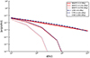 |
Fig. A.1. Comparison of the simulated radio emission spectra for a source with an input α = 0.6 radio spectrum and with a constant B = 10 μG uniform magnetic field, evolved using our cosmic ray electron solver, or using using BRATS (Harwood et al. 2015). |
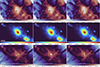 |
Fig. A.2. Maps of projected mass weighted mean gas temperature (top row), total X-ray emission in the [0.5-2 keV band (middle row), and projected mass weighted mean magnetic field strength (bottom row) at z = 0.391 for our three resimulations of jets with Pj = 4 × 1044 erg/s power, with jets expanding either along the x, y, or z axis of the simulation. Each panel has size 4.2 ×3.2 Mpc. |
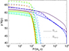 |
Fig. A.3. Evolution of the relativistic electron spectra in the innermost ≤300 kpc of our cluster in the run E model and including all loss and gain terms, using the rescaled magnetic field as in the main text (solid lines) or the original magnetic field produced by the MHD simulation (dashed lines). The different colours mark 10 different epochs, roughly equally spaced in time, from z = 0.5 (black) to z = 0.1 (red). |
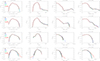 |
Fig. A.4. Distributions of gas density, gas temperature, velocity dispersion, and magnetic field strength for four epochs, comparing different prescriptions for the jet model in run D (see text for explanations). The distributions are taken within a reference comoving 13 Mpc3 around the (moving) cluster center of mass at four different redshifts. |
Appendix B: Tests with the original magnetic field of the simulation
As explained in Section 2.7, the spatial resolution obtained with these runs is not enough to ensure a realistically large Reynolds number across the simulated ICM volume, which prevents the amplification of the cluster magnetic field by the small-scale dynamo (e.g. Mingo et al. 2022). We therefore evolved our relativistic electrons under the effect of a re-normalised magnetic field, extrapolated based on the local measured value of the solenoidal turbulent energy flux, and assuming a fixed conversion of this energy flux (2%) into the creation of new magnetic field (e.g. Beresnyak & Miniati 2016; Vazza et al. 2018).
In Figure A.3, we show the simulated electrons spectra for the innermost (≤300 kpc) region of our group in the run E model and using all loss and gain terms, obtained either with the rescaled magnetic field as in the main paper (Bturb), or with the original magnetic field directly produced by the MHD simulation (BMHD). As commented already in the main paper, the average difference in the magnetic field across the tracer distribution is not dramatic, that is, ⟨Bturb⟩∼2 − 3⟨BMHD⟩. However, the difference can be more significant for those tracers sampling spectra in very turbulent regions, and these differences can be amplified in simulated spectra, as the can crucially affect the balance between synchrotron losses (which scales as ∝B−2) and the turbulent re-acceleration term (which scales as ∝B, see Equation 11).
For this reason, if turbulent re-acceleration is considered in combination with an unrealistically low magnetic field, an unrealistically large amount of low energy electrons can be re-accelerated. This is clearly shown by Figure A.3, where we can see the progressive buildup of the electron distribution at p ≤ 104, leading to a final excess of order ∼102 − 103 in the total energy of fossil relativistic electrons, compared to our more realistic choice of the rescaled magnetic field, Bturb. Since this also leads to the overproduction of low-frequency radio emission in our galaxy group, we consider the rescaled magnetic field a better option to obtain a realistic view of the evolving population of fossil electrons in the ICM.
Appendix C: Tests with additional physical variations
While our main paper focuses on the influence of the initial power of jets on the long-term evolution of gas and electrons in a reference group of galaxies, additional differences can be expected for different choices in the initial direction of jets. Therefore, we produced two additional resimulations of the intermediate case of run D in which we released exactly the same power (Pj = 4 × 1044 erg/s) along the other other two possible perpendicular directions: run Dy and Dx. These are meant to explore whether the large scale circulation of injected electrons can show different properties, depending on the different sectors in the ICM the jets expand into, and in the possible different amount of frustration that jets can experience depending on the ICM flow they encounter. Figure A.2 gives the projected view of the three simulations after 1 Gyr since the jet injection (showing minimal differences between runs, with the obvious exception of the cluster core), while Figure A.4 shows that no significant differences in the statistics of the thermodynamical properties of the ICM are seen in the three runs, indicating that our main results are not affected by jet orientations. With run coolD, we also tested whether the evolution of the cluster after the jet injection can be affected by radiative cooling, which is switched on in this case: again, with the exception of small tail of low temperature gas (T ≤ 106 K) forming at low redshift in the latter case, we report that the main finding of our paper are unchanged. Future works will focus on investigating the more realistic case of having cooling active from the start of the simulation, which can potentially leading to multi-phase ICM and to a higher level of gas clumping and interacting with jets.
All Tables
Best-fit parameters for the relation between the average distance covered by tracers and the input jet power, for five different epochs.
All Figures
|
Fig. 1. RGB rendering of the evolution of thermal gas and passive tracers (marking relativistic electrons injected by jets) in our runs. The red colour marks the density of passive tracers, the blue the gas temperature and the green the X-ray emission. Each panel has a side of 5.5 Mpc (comoving). |
| In the text | |
|
Fig. 2. Evolution of the median of comoving gas density, magnetic field strength, temperature, Mach number (only for shocked tracers), module of vorticity, and divergence measured by tracers in all our runs with jets. The time is measured since the start of the jets launching, i.e. from z = 0.5. In the upper right plot, we show with solid lines the trend of the original magnetic field produced by our MHD simulation, while the dotted lines display the rescaled magnetic field value, based on the local turbulent field, as estimated in Sect. 2.7. |
| In the text | |
|
Fig. 3. Distributions of gas density, gas temperature, velocity dispersion, and magnetic field strength for four epochs, for a reference comoving 13 Mpc3 around the (moving) cluster center of mass at four different redshifts. For comparison, we also report the distributions from the Run 0, without jets (grey lines). |
| In the text | |
|
Fig. 4. Evolution of the median distance travelled by tracers in all runs, either with respect to the particle center of mass at all epochs (left panel), or with respect to their initial injection site (right panel). The time is measured since the start of the jets launching, i.e. from z = 0.5. |
| In the text | |
|
Fig. 5. Relation between the average distance reached by tracers in four different epochs, as a function of the input jet power in the five runs. The time is measured since the start of the jets launching, i.e. from z = 0.5. |
| In the text | |
|
Fig. 6. Projected number of relativistic electrons within the same column of cells along the line of sight in run D (top), and radio emission at 50 MHz at four different epochs, in the electron model including all loss and re-acceleration terms. The blue contours in the lower raw show the regions potentially detectable with LOFAR LBA. |
| In the text | |
|
Fig. 7. Evolution of the momentum distributions of electrons in the run D, for five different epochs and for the three different acceleration and cooling models (colours). The dashed lines are referred to the cluster region r ≤ 300 kpc while the solid lines are for electrons at any distance from the cluster centre. |
| In the text | |
|
Fig. 8. Projected number of relativistic electrons in run E (top) and radio emission at 50 MHz at four different epochs, in the electron model including all loss and re-acceleration terms. The blue contours in the lower raw show the regions potentially detectable with LOFAR LBA. |
| In the text | |
|
Fig. 9. Projected number of relativistic electrons in run F (top) and radio emission at 50 MHz at four different epochs, in the electron model including all loss and re-acceleration terms. The blue contours in the lower raw show the regions potentially detectable with LOFAR LBA. |
| In the text | |
|
Fig. 10. Momentum distributions of electrons at z ≈ 0.39 in our five runs (i.e. ≈760 Myr after the jet injection), for the three different acceleration or cooling models (colours). The dashed lines are referred to the cluster region r ≤ 300 kpc while the solid line (here overlapping with the first) are for electrons at any distance from the cluster centre. The lowest power run B is at the top and the highest power run F is at the bottom. |
| In the text | |
|
Fig. 11. Momentum distributions of electrons at z = 0.13 in our five runs (i.e. ≈3.2 Gyr after the jet injection), for the three different acceleration or cooling models (colours) and marking the core cluster region r ≤ 300 kpc (dashed) or the entire cluster volume (solid). The lowest power run B is at the top and the highest power run F is at the bottom. |
| In the text | |
|
Fig. 12. Distributions of the ratio between the total energy of all relativistic electrons we evolved in our runs at four different epochs, and the thermal gas energy associated with the same tracers. The solid lines give the distribution of Ecr/Eg for the electron evolution model including shocks and turbulent re-acceleration, while the dashed lines are for the electron model only including radiative losses and adiabatic changes after the injection by jets. |
| In the text | |
|
Fig. 13. Distributions of the ratio between the total energy of all relativistic electrons we evolved in our runs at four different epochs, and the thermal gas energy associated with the same tracers. The solid lines give the distribution of Ecr/Eg for the electron evolution model including shocks and turbulent re-acceleration, while the dashed lines are for the electron model only including radiative losses and adiabatic changes after the injection by jets. This figure only includes P/(mec)≥103 electrons in the computation of Ecr. |
| In the text | |
|
Fig. 14. Evolution of the synchrotron radio spectra of all electrons in the run D, for ten different epochs. The solid lines are the spectra including all loss and re-acceleration terms, the dashed line are for models including all loss terms and shock (re)acceleration, while the dotted lines are for models that include only loss terms. |
| In the text | |
|
Fig. 15. Synchrotron radio spectra in our five runs at z = 391 (i.e. ≈760 Myr after the jet injection) and at z = 0.142 (≈3.2 Gyr after the jet injection). The solid lines are the spectra including all loss and re-acceleration terms, the dashed line are for models including all loss terms and shock (re)acceleration, while the dotted lines are for models including only loss terms. |
| In the text | |
|
Fig. 16. Distributions of radio spectral index between 140 and 50 MHz, only for ≥1σrms detectable pixels in radio maps of the run E at four different epochs. The solid lines give the distribution of distribution of spectra for the electron evolution model including shocks and turbulent re-acceleration, the dashed lines are for the electron model only including shock re-acceleration and loss terms, and the dotted lines are for the electron model only including radiative losses and adiabatic changes after the injection by jets. |
| In the text | |
|
Fig. 17. Distributions of radio spectral index between 140 and 50 MHz, only for ≥1σrms detectable pixels in radio maps of all runs at four different epochs, only for the electron evolution model including all loss and re-acceleration terms. |
| In the text | |
|
Fig. 18. Evolution of the total radio emission within ≤500 kpc from the group centre at 140 MHz, as a function of the X-ray emission in the [0.5−2] keV range within the same region, from z = 0.5 to z = 0.4 and for our five runs. The top panel shows our prediction for a model in which electrons are injected by jets and are then only subject to radiative and adibatic changes, while in the lower panel all re-acceleration mechanisms are considered. The grey points show the real LOFAR-HBA and eRosita observations from Pasini et al. (2022). |
| In the text | |
|
Fig. A.1. Comparison of the simulated radio emission spectra for a source with an input α = 0.6 radio spectrum and with a constant B = 10 μG uniform magnetic field, evolved using our cosmic ray electron solver, or using using BRATS (Harwood et al. 2015). |
| In the text | |
|
Fig. A.2. Maps of projected mass weighted mean gas temperature (top row), total X-ray emission in the [0.5-2 keV band (middle row), and projected mass weighted mean magnetic field strength (bottom row) at z = 0.391 for our three resimulations of jets with Pj = 4 × 1044 erg/s power, with jets expanding either along the x, y, or z axis of the simulation. Each panel has size 4.2 ×3.2 Mpc. |
| In the text | |
|
Fig. A.3. Evolution of the relativistic electron spectra in the innermost ≤300 kpc of our cluster in the run E model and including all loss and gain terms, using the rescaled magnetic field as in the main text (solid lines) or the original magnetic field produced by the MHD simulation (dashed lines). The different colours mark 10 different epochs, roughly equally spaced in time, from z = 0.5 (black) to z = 0.1 (red). |
| In the text | |
|
Fig. A.4. Distributions of gas density, gas temperature, velocity dispersion, and magnetic field strength for four epochs, comparing different prescriptions for the jet model in run D (see text for explanations). The distributions are taken within a reference comoving 13 Mpc3 around the (moving) cluster center of mass at four different redshifts. |
| In the text | |
Current usage metrics show cumulative count of Article Views (full-text article views including HTML views, PDF and ePub downloads, according to the available data) and Abstracts Views on Vision4Press platform.
Data correspond to usage on the plateform after 2015. The current usage metrics is available 48-96 hours after online publication and is updated daily on week days.
Initial download of the metrics may take a while.