| Issue |
A&A
Volume 655, November 2021
|
|
|---|---|---|
| Article Number | A59 | |
| Number of page(s) | 53 | |
| Section | Stellar structure and evolution | |
| DOI | https://doi.org/10.1051/0004-6361/202141572 | |
| Published online | 19 November 2021 | |
Detection of non-linear resonances among gravity modes of slowly pulsating B stars: Results from five iterative pre-whitening strategies
1
Institute of Astronomy, KU Leuven, Celestijnenlaan 200D, 3001 Leuven, Belgium
e-mail: jordan.vanbeeck@kuleuven.be
2
Kavli Institute for Theoretical Physics, University of California, Santa Barbara, CA 93106, USA
3
Reference Systems and Planetology, Royal Observatory of Belgium, Brussels, Belgium
4
Dept. of Astrophysics, IMAPP, Radboud University Nijmegen, 6500 GL Nijmegen, The Netherlands
5
Max Planck Institute for Astronomy, Koenigstuhl 17, 69117 Heidelberg, Germany
Received:
16
June
2021
Accepted:
5
August
2021
Context. Slowly pulsating B (SPB) stars are main-sequence multi-periodic oscillators that display non-radial gravity modes. For a fraction of these pulsators, 4-year photometric light curves obtained with the Kepler space telescope reveal period spacing patterns from which their internal rotation and mixing can be inferred. In this inference, any direct resonant mode coupling is usually ignored.
Aims. We re-analyse the light curves of a sample of 38 known Kepler SPB stars. For 26 of them, the internal structure, including rotation and mixing, was recently inferred from their dipole prograde oscillation modes. Our aim is to detect direct non-linear resonant mode coupling among the largest-amplitude gravity modes.
Methods. We extract up to 200 periodic signals per star with five different iterative pre-whitening strategies based on linear and non-linear regression applied to the light curves. We then identify candidate coupled gravity modes by verifying whether they fulfil resonant phase relations.
Results. For 32 of the 38 SPB stars we find at least one candidate resonance that is detected in both the linear and the best non-linear regression model fit to the light curve and involves at least one of the two largest-amplitude modes.
Conclusions. The majority of the Kepler SPB stars reveal direct non-linear resonances based on the largest-amplitude modes. These stars are thus prime targets for the non-linear asteroseismic modelling of intermediate-mass dwarfs to assess the importance of mode couplings in probing their internal physics.
Key words: asteroseismology / stars: oscillations / stars: early-type / stars: variables: general / stars: rotation / methods: data analysis
© ESO 2021
1. Introduction
Three decades ago Waelkens (1991) first coined the term ‘slowly pulsating B’ (SPB) stars to describe mid-B variable stars that display low-frequency oscillations with physical properties similar to 53 Persei variables (see e.g. Waelkens & Rufener 1985, and references therein). The SPB stars are mid-to-late B main-sequence (MS) stars with masses ranging from ∼3 to ∼9 M⊙ (De Cat & Aerts 2002; Aerts et al. 2010; Pedersen et al. 2021) and displaying all levels of rotation, from very slow up to the critical rotation rate (Pedersen et al. 2021). A distinct feature is their multi-periodic photometric and spectroscopic variability, with periods typically ranging from ∼0.5 to ∼5.0 d and amplitudes of typically less than ∼10 mmag (e.g. Aerts et al. 2010; Pápics et al. 2017; Pedersen et al. 2021). Their variability was attributed to low-degree, high-radial-order gravity (g) modes, which are excited by the heat engine (i.e. κ) mechanism driven by an opacity enhancement from the iron-group elements, also called the Z Bump, at a temperature of ∼200 000 K (Gautschy & Saio 1993; Dziembowski et al. 1993; Pamyatnykh 1999).
The oscillations in SPB stars were already fairly well characterised from ground-based photometric and spectroscopic observations (e.g. Aerts et al. 1999; De Cat et al. 2000, 2005, 2007; Mathias et al. 2001; De Cat & Aerts 2002), but their asteroseismic potential became clear when CoRoT (‘Convection, Rotation and planetary Transits’; Auvergne et al. 2009) and Kepler (Borucki et al. 2010) space photometry became available (see e.g. Degroote et al. 2010; Balona et al. 2011, 2015; Pápics et al. 2012, 2014, 2015; Pápics et al. 2017; Szewczuk & Daszyńska-Daszkiewicz 2018; Pedersen et al. 2021; Szewczuk et al. 2021, for recent examples of light curves). Because of their wealth in number of excited and identified oscillation modes, they have been the target of various asteroseismic modelling efforts in the past few years, which focused on inferring the internal mixing and rotation (e.g. Moravveji et al. 2015, 2016; Triana et al. 2015; Pápics et al. 2017; Pedersen et al. 2021; Michielsen et al. 2021) and on mode excitation (e.g. Szewczuk & Daszyńska-Daszkiewicz 2018; Szewczuk et al. 2021). There have also been efforts to characterise the magnetic field of a small number of SPB stars by analysing the frequency shifts of its g modes (e.g. HD 43317, Buysschaert et al. 2018; Prat et al. 2019, 2020). The influence of rotation on the g modes in SPB stars is more important than the magnetic shifts and implies that almost all modes are in the gravito-inertial regime (Aerts et al. 2017, 2019). The effects of rotation, therefore, cannot be incorporated from a perturbative treatment of the Coriolis acceleration, which leads many authors to adopt the so-called traditional approximation of rotation (TAR; see e.g. Longuet-Higgins 1968; Lee & Saio 1997; Townsend 2003; Degroote et al. 2009a; Mathis 2013) for pulsation computations (e.g. Szewczuk & Daszyńska-Daszkiewicz 2018; Pedersen et al. 2021; Szewczuk et al. 2021; Michielsen et al. 2021).
Rapid rotation also deforms a star, causing it to become oblate. The rotation rates of SPB stars cover the cases from slight to major deformation. However, the detected and identified modes have their dominant mode energy deep inside the star, close to the convective core, where spherical symmetry still applies well. This justifies a treatment of g modes in the TAR (Mathis & Prat 2019; Henneco et al. 2021; Dhouib et al. 2021). An important consequence of the rapid rotation of some SPB stars is the occurrence of mode coupling between over-stable convective modes based on frozen-in core convection and envelope g modes excited by the κ mechanism (Lee 2021).
Slowly pulsating B stars have so far been modelled from linear pulsation theory. Period spacing patterns constructed from the frequencies of identified g modes of consecutive radial order and the same angular degree and azimuthal order are the most important tool used in linear asteroseismic modelling. Such patterns can display oscillatory features that were found to be attributable to chemical gradients inside the star (e.g. Miglio et al. 2008). Moreover, they display a slope due to the rotation rate near the convective core (e.g. Bouabid et al. 2013; Pápics et al. 2017). Some SPB stars, however, can show structure in their g-mode period spacing patterns that is hard to explain without incorporating additional physical effects into the oscillation model, such as rotational deformation (e.g. Dhouib et al. 2021), (internal) magnetism (see e.g. Van Beeck et al. 2020), or resonances of envelope g modes with inertial modes in the core (e.g. Ouazzani et al. 2020; Saio et al. 2021).
The inputs to asteroseismic modelling based on linear oscillation theory are the independent frequencies extracted from an observed time series (e.g. a light curve), where frequency extraction is usually done using an iterative pre-whitening procedure (e.g. Degroote et al. 2009a). However, non-sinusoidal light curves give rise to harmonics and combination frequencies (dependent frequencies) in the amplitude spectrum (Pápics 2012; Kurtz et al. 2015). These combination frequencies are therefore also included in the extracted frequencies. The phases and amplitudes of the independent frequencies, as well as the frequencies, amplitudes, and phases of the combination frequencies, are subsequently neglected during linear asteroseismic modelling. On the other hand, frequency perturbations within g-mode period spacing patterns are expected if non-linear mode coupling is accounted for (e.g. Buchler & Goupil 1984; Van Hoolst 1996). Hence, this may be an alternative explanation for the deviations in the period spacing patterns of SPB stars. Such frequency shifts may be small if the g modes are only moderately non-linear, as was the case for most ‘well-observed’ non-radial pulsators such as white dwarfs or δ Sc stars (Buchler et al. 1997); however, this remains to be verified for SPB stars.
As detailed in Buchler et al. (1997), resonances among (excited) non-radial oscillation modes also play an important role in mode selection and interaction and can lead to additional constraints on mode identification. Resonant interactions among modes can further hamper pattern identification due to so-called frequency or phase locking. This complication of pattern identification originates from the fact that the exact resonance relation, ∑ini ωi = 0, need not be satisfied for linear mode frequencies. It suffices that linear mode frequencies are in near resonance, such that the exact resonance relation between angular frequencies ωj is satisfied, aside from a small angular frequency difference δω. Non-linear frequency shifts can then lead to a non-linear frequency locking or phase locking, where the non-linear locked frequencies satisfy the resonance condition exactly, which can distort the period spacing patterns relied upon in linear asteroseismology.
The theoretical framework of resonant mode coupling, the amplitude equation (AE) formalism, was described in numerous publications (e.g. Dziembowski 1982; Buchler & Goupil 1984; Dziembowski & Krolikowska 1985; Buchler 1993; Buchler et al. 1997; Van Hoolst & Smeyers 1993; Van Hoolst 1994a,b, 1995). It has the inherent validity assumption that the (linear) growth rates, γ, of the modes are small compared to their angular frequencies, which is generally assumed to be satisfied for observed MS oscillators (see e.g. Barceló Forteza et al. 2015; Bowman et al. 2016). The AEs constitute a set of coupled first-order complex non-linear ordinary differential equations and predict the temporal behaviour of the mode amplitudes and phases. Three main regimes of mode interaction are distinguished (as was explained in Buchler et al. 1997).
First, if two or more modes are close to being in resonance, such that Dg ≡ δω/γ is of order 1 or smaller (where δω is the angular frequency mismatch or angular frequency de-tuning), and a stable fixed point (FP) solution exists for the AEs, for which the mode amplitudes and phases are constant over time, the frequencies are locked. These locked frequencies can be substantially different from their non-resonant counterparts.
Second, with an increasing angular frequency mismatch, δω, the FP solution becomes unstable or disappears and a bifurcation to another solution takes place, with amplitude (and phase) modulation. The larger the value of Dg, the smaller the amplitude of the modulation. Goupil et al. (1998) called this bifurcating regime the ‘intermediate’ regime.
Third, at large δω one encounters the solution where frequencies are approximately equal to their (unlocked) non-resonant values. The non-linear non-resonant frequencies have a small frequency shift compared to their linear counterparts: This is the mildly non-linear regime in which linear asteroseismology operates. Goupil et al. (1998) called this the ‘non-resonant’ regime.
In addition, a narrow hysteresis (transitory) regime exists in between the frequency-locked and intermediate regimes, in which amplitudes are modulated but frequencies (or equivalently, phases) remain constant (Buchler et al. 1997).
The study of the relationships among amplitudes and phases, which provide the observables to be matched to the theoretical predictions from the AEs, is a standard approach for the analysis of light curves of RR Lyr stars and Cepheids (as pioneered by Simon & Lee 1981). It is also a well-established technique for unravelling non-linearities in the light curves of oscillating white dwarf stars (e.g. Wu 2001; Zong et al. 2016a) and hot B subdwarf stars (e.g. Zong et al. 2016b). Yet, it receives not much attention for oscillating MS stars (Lee 2012; Bowman & Kurtz 2014; Kurtz et al. 2015; Bowman et al. 2016, 2021).
In this work, we provide the identification of candidate direct resonances among the extracted oscillation frequencies in the light curves of 38 SPB stars and test the impact of different iterative pre-whitening strategies on the results. In Sect. 2 we summarise the characteristics of our sample, the strategies we employ to analyse the light curves, and discuss how we search for candidate direct resonances. We discuss the light curve analysis strategy selection process in Sect. 3 and the results of the candidate resonance search in Sect. 4. A summary of our conclusions and future prospects can be found in Sect. 5.
2. Light curves and their analysis
2.1. The Pedersen (2020) SPB sample
Our sample consists of 38 stars originally identified as SPB stars based on Kepler photometry (Balona et al. 2011, 2015; McNamara et al. 2012; Pápics et al. 2013, 2014, 2015; Pápics et al. 2017; Zhang et al. 2018; Szewczuk & Daszyńska-Daszkiewicz 2018). We use the light curves extracted from the 30-min cadence target pixel data by Pedersen (2020), who used customised pixel masks (see Pápics et al. 2017 for further details). After light curve extraction, Pedersen (2020) manually removed outliers, and separately corrected each quarter for instrumental trends by fitting a low-order polynomial to the data. Pedersen (2020) then converted the light curves to have flux units of ppm, and normalised them to have an average flux of zero.
Contrary to previous analyses of Kepler SPB stars by Szewczuk & Daszyńska-Daszkiewicz (2018), Pedersen (2020), Szewczuk et al. (2021) and Pedersen et al. (2021), we use five different iterative pre-whitening strategies, each of which produce a final regression model fit for the light curve. Our approach is motivated by the fact that iterative pre-whitening techniques vary in the literature, while it is not assessed how these various approaches influence frequency extraction results. Our comparative capacity assessment of the different iterative pre-whitening procedures is an important aspect of the hunt for non-linear resonances in SPB stars.
2.2. SPB light curve analysis
We employ five pre-whitening strategies to derive frequencies, amplitudes and phases from the light curves, which emulate various approaches taken in the literature. The first timestamp of each light curve was subtracted from all timestamps of that light curve to provide a consistent zero point in time for phase calculation. Strategy 1 uses a non-linear least-squares fit of the entire multi-parameter model in the time domain at each pre-whitening step (Bowman et al. 2016). It requires each signal to have an amplitude S/N ≥ 4 (Breger et al. 1993) computed in a window of 1 d−1 around the target frequency and it fits a model comprising a sum of sinusoids, F(ti), to the light curve,
![$$ \begin{aligned} F(t_i) = \beta _0 + \sum _{j=1}^{n_{\rm f}} A_j \sin \left[2\pi \nu _j t_i + \phi _j\right], \end{aligned} $$](/articles/aa/full_html/2021/11/aa41572-21/aa41572-21-eq1.gif)
for each ti, i = 1, …, nt, with nt the total number of timestamps of the light curve. In this expression, nf is the number of fitted frequencies, β0 is the y intercept, Aj denotes the amplitude, νj(≡ωj/2π) is the temporal frequency, and ϕj is the phase of fitted sinusoid j. The other four pre-whitening strategies differ from this first one in the way they determine the initial parameters for the optimisation (i.e. parameter hinting; see the notes of Table 1), stop criterion, and whether a linear or non-linear (multi-parameter) least-squares optimisation is performed at the end of each iterative pre-whitening step. These differences are listed in Table 1.
Five iterative pre-whitening strategies employed in this work.
As is commonly done, we calculate the uncertainties for the extracted parameters, under the assumption that they are uncorrelated, using
where σnt is the standard deviation of the residual signal (after the regression model has been subtracted from the light curve), Â is the optimised amplitude, T is the total time span of the data, and where D is a correction factor for the correlated nature of the light curve data, which can be estimated as the square root of the average number of consecutive data points of the same sign in the residual light curve (e.g. Schwarzenberg-Czerny 1991, 2003; Montgomery & O’Donoghue 1999; Degroote et al. 2009a).
During each pre-whitening step we compute the Lomb-Scargle (LS) periodogram (Lomb 1976; Scargle 1982) of the (residual) light curve, with frequency grid step equal to 0.1 ℜν (where  is the Rayleigh limit). The start and end values of this frequency grid are equal to 1.5 ℜν and the Nyquist frequency νNyq (
 , where
  is the median cadence of the time series), respectively. The LS periodogram, together with a specific parameter hinting rule listed in Table 1, are used to provide the preliminary amplitude and frequency hint, taking into account the frequency resolution (Loumos & Deeming 1978), hereafter referred to as the LD78 resolution. The preliminary phase hint is subsequently obtained from a linear least-squares fit to the residual light curve, where frequencies and amplitudes in Eq. (1) are fixed at either their frequency and amplitude hint values (the frequency being extracted) or the values they had in the previous pre-whitening step (all other frequencies). The phase hinting optimisation employs the Trust-region reflective least-squares regression method implemented in the Python package LMFIT (Newville et al. 2020), whose exact configuration is specified in Appendix A. For strategies 1 to 4 the optimised parameter hints are then fed to the non-linear least-squares optimiser at the end of this pre-whitening step to optimise the frequencies, amplitudes and phases of the entire model. For strategy 5, however, these parameter hints are only used in a linear least-squares optimisation of the amplitudes and phases, where the frequencies are fixed at the values determined from an over-sampled LS periodogram in a 1 d−1 region around the preliminary frequency hint (signal extracted during this iterative pre-whitening step), and the values they had in the previous iteration step (other signals). The Levenberg–Marquardt method implemented in LMFIT (Newville et al. 2020) is used for this optimisation, whose exact configuration is specified in Appendix A.
Each iterative pre-whitening process continues until 200 frequencies are extracted in this way, or until the specified stop criterion as in Table 1 is reached. After the frequency extraction, we verify that the amplitude of each extracted frequency is significant at the 95% level using a Z-test, whilst taking the LD78 resolution into account. If at least one insignificant extracted frequency is detected, the last extracted insignificant frequency is removed. After that frequency is removed, the entire model is re-optimised, and a new significance check is performed. This iterative process, which we refer to as the frequency filtering step, continues until no further insignificant frequencies occur in the regression model.
The regression models for each of the pre-whitening strategies that have undergone frequency filtering are then compared with one another. To quantify the quality of the regression model, we rely on the residual sum of squares, weighted by the total variance in the observed light curve and by a factor including the total number of free parameters of the regression model, np, versus nt. To end up with a maximum likelihood estimator, we subsequently use the scaled fraction of variance, fsv, which we define as
where yi denotes the time series signal at timestamp ti, and 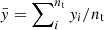 is the mean signal of the time series. The higher the quality of the regression model, the closer fsv approaches unity while we punish for a higher number of free parameters.
2.3. Candidate resonant Kepler SPB oscillations
In our identification of direct resonant mode interactions we focus on FP solutions of the AEs, for which frequency locking persists (Buchler et al. 1997). Any such solutions have parent-daughter frequency combinations that approximately satisfy the (direct) resonance relation. Our aim is to extract information on the least complicated mode interactions, and hence we use strict candidate resonance identification criteria. The first criterion requires that a frequency combination of a candidate resonance satisfies the following relation:
where νdaughter is the daughter frequency, νparent, i is its ith parent frequency, ni ∈ ℤ, and where δν is the frequency de-tuning, for which |δν|< νdaughter holds. This follows the parent-daughter terminology introduced in Degroote et al. (2009a). To further characterise and verify the direct candidate resonance, and following Buchler et al. (1997), Vuille (2000) and Vuille & Brassard (2000), we compute relative phases and amplitudes. The second candidate resonance identification criterion then consists of verifying whether the corresponding relative phases Φ of the combinations that satisfy Eq. (4) also satisfy the following (resonant) relative phase relation (see e.g. Fig. 13 in Van Hoolst 1995, in which Γ0 and σ denote the FP relative phase and frequency de-tuning, respectively, as well as Fig. 1 in Buchler et al. 1997):
![$$ \begin{aligned} \exists k \in \left[-4,\,-3,\,\ldots ,\,4\right]:\Phi \equiv \phi _{\rm daughter} - \sum _i n_i\,\phi _{\mathrm{parent},\,i} \approx k\cdot \dfrac{\pi }{2}, \end{aligned} $$](/articles/aa/full_html/2021/11/aa41572-21/aa41572-21-eq9.gif)
where ϕdaughter is the extracted phase of the daughter frequency, and ϕparent, i is the extracted phase of its ith parent frequency. If for a given candidate combination of parent(s) and daughter frequencies Eqs. (4) and (5) are satisfied, this pair is classified as a candidate resonance. We define the combination order o of this candidate resonance as: o = ∑i|ni|. Following Vuille & Brassard (2000) we compute the relative amplitude of the candidate resonance, Ar, in the following way:
In practice, we limit ourselves to identifying up to second-order combinations of parent frequencies (o = 2). For each potential candidate direct resonance, we then verify whether Eq. (4) is satisfied to within 1 Rayleigh limit ℜν at the 1σ level:

where ν ≡ ∑ini νparent, i is a combination frequency composed of other extracted frequencies, with propagated uncertainty σν. The comparison with ℜν hence measures whether ν is resolved with respect to νdaughter. We used this practical approximation for assigning candidate resonance identifiers, to avoid use of the theoretical criterion by Buchler et al. (1997), |δω|/γ ≲ O(1), setting the approximate limits of parameter space for which an FP solution with frequency locking exists, as it relies on model-dependent non-adiabatic oscillation calculations for γ, while we wanted to establish a data-driven approach. If Eq. (7) holds, we further verify whether the relative phase Φ of the candidate combination satisfies Eq. (5) to within 1σ:
![$$ \begin{aligned} \exists k \in \left[-4,\,-3,\,\ldots ,\,4\right]: \Phi - \sigma _\Phi \le k \cdot \dfrac{\pi }{2} \le \Phi + \sigma _\Phi . \end{aligned} $$](/articles/aa/full_html/2021/11/aa41572-21/aa41572-21-eq12.gif)
3. Results: Light curve regression model capacity
In this section the resulting regression models obtained for each of the five pre-whitening strategies applied to all 38 stars in our sample are compared. The metrics used for this comparison are the fsv value defined in Eq. (3), the (residual) light curves and their LS periodogram. The fsv metric measures how well the five regression models describe the light curve of any given star, where we recall that Eq. (1) assumes that each oscillation mode has constant amplitude, frequency, and phase. Under this assumption and using the criteria in Table 1, we define the best regression model as the one with the highest fsv. Any violation of the assumed constant amplitudes, phases, or frequencies results in lower values of fsv along with the occurrence of more harmonics and combination frequencies.
Based on the fsv metric, we divide the stars in our sample into two pseudo-classes: (i) stars for which the light curve regression models attain fsv values above 0.9 after frequency filtering for all five iterative pre-whitening strategies; and (ii) stars for which at least one of these models attains a value of fsv < 0.9. For brevity, we instead refer to strategies ‘having’ fsv values above 0.9 in the remainder of the text. This classification accentuates the apparent bimodality in the distribution of the fsv metric values that can be seen in Fig. 1. Half of the 38 SPB stars in our sample have fsv ≥ 0.9 for all five pre-whitening strategies and thus belong to pseudo-class 1, hereafter referred to as the ‘high-fsv’ stars. We discuss their light curve regression model selection process in Sect. 3.1. We additionally subdivide the stars belonging to the second pseudo-class (the ‘low-fsv’ stars) into two additional pseudo-classes based on whether outburst-like features are detected in the light curves, and thus end up with three pseudo-classes that describe the whole sample. The light curve regression model selection process for these two additional pseudo-classes, the high-mode-density stars and the outbursting stars, are discussed in Sect. 3.2, both guided by particular example stars. The percentages of explained scaled variance fsv averaged over all stars in our sample, and averaged over the stars belonging to each of these pseudo-classes are shown in Fig. 2. According to this ‘sample’ metric, high-fsv stars are explained well by the regression models belonging to the five pre-whitening strategies. However, significantly differing values of fsv can be noted for low-fsv stars. For the sample of 38 SPB stars as a whole, the overall highest-fsv regression model is the one delivered by pre-whitening strategy 3, as will be discussed further below. The best regression model and other properties for all individual stars in our sample are discussed in Appendix B.
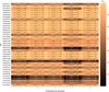 |
Fig. 1. Comparison of the scaled fraction of variance fsv values of the resulting light curve regression models obtained for the different pre-whitening strategies applied to the stars in the sample, with colouring as a function of fsv. Each cell contains the fsv value as computed using Eq. (3), as well as the total number of frequencies extracted using this approach, ne. The number ne and the fsv value are computed after the frequency filtering step has removed any unresolved frequencies with respect to the LD78 criterion and any signals that have insignificant amplitudes (at 95% confidence), as discussed in Sect. 2.2. |
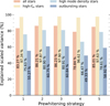 |
Fig. 2. Total percentage of explained scaled variance fsv averaged over all 38 stars in the sample (‘all stars’) for each of the five pre-whitening strategies. This averaged percentage is also displayed for each of the three pseudo-classes introduced in Sect. 3. |
3.1. High-fsv stars
We discuss the light curve regression model selection process for high-fsv stars guided by the example of KIC005941844, classified as an SPB star by McNamara et al. (2012) and analysed by Pedersen (2020) and Pedersen et al. (2021). Its light curve is well explained by sinusoids of constant amplitude and frequency, as demonstrated by the high fsv values shown in Fig. 1 and the light curve in the top panel of Fig. 3. The light curves of high-fsv stars are, in general, (nearly) sinusoidal, because a large degree of variance is explained by the model generated by Eq. (1). The most prominent data gaps in the light curve of KIC005941844 are caused by the loss of Kepler’s charge-coupled device (CCD) module 3, one year into the mission.
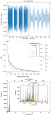 |
Fig. 3. Light curve, pre-whitening and pulsation characteristics for the high-fsv star KIC005941844. Top: full light curve (left) and a small part of the light curve that indicates its multi-periodic constant-frequency nature (right). Middle: comparison of the different stop criteria used for the five pre-whitening strategies throughout the iterative pre-whitening procedure, applied to the light curve. The BIC values are relevant for strategies 3, 4, and 5, whereas the S/N value and the estimated amplitude A expressed in estimated standard deviations |

The middle panel of Fig. 3 shows a comparison of the values of the metrics important for the stop criteria of all five strategies, throughout the iterative pre-whitening process. The values of these metrics as a function of the pre-whitening step number indicate the progress of that process before frequency filtering is carried out, and are henceforth referred to as the ‘iteration progress curves’. If the gradient of the Bayesian information criterion (BIC) iteration progress curve (strategy 3, 4, or 5) converges to a value of zero, the regression model is approaching the optimal model according to the likelihood ratio test (LRT). The LRT compares the nested light curve regression models of this and the previous step based on the likelihoods inferred from the BIC values. A significant upward trend in the BIC iteration progress curve increases the p-value of the LRT to a value greater than the stop criterion, with the significance of that trend depending on the difference in BIC values and number of optimisation parameters of the nested regression models. The S/N iteration progress curve (strategy 1) represents the signal-to-noise ratio of the frequency extracted during each iterative pre-whitening step. If it falls below the pre-set limit S/N = 4.0 (Breger et al. 1993), the stop criterion is triggered and iterative pre-whitening stops. Finally, the  iteration progress curve represents the amplitude of the frequency extracted during each iterative pre-whitening step, in terms of its standard deviation. Iterative pre-whitening for strategy 2 is stopped if the amplitude of the frequency extracted is consistent with 0.0 ppm at 95% confidence level (i.e.
  ).
).
The iteration progress curves provide a metric that dictates whether a light curve regression model is nearing its optimal parameters. This needs to be investigated on a star-to-star basis, because it intrinsically depends on the oscillation mode density in the (residual) LS periodograms and amplitudes attained by any of the periodic signals in the light curves. For KIC005941844, the iteration progress curves indicate that for all five iterative pre-whitening strategies, the optimal or near-optimal model has been obtained, before any additional post-processing frequency filtering. The frequency filtering step removes unresolved frequencies and frequencies that do not have significant amplitudes (at a 95% confidence level), so that the final light curve regression models are obtained. The numbers of frequencies retained in the regression models after this frequency filtering step (i.e. the numbers of final resolved significant extracted frequencies) are indicated in Fig. 1 by the ne parameter for each strategy applied to the light curve of each star.
The differences among the fsv values of the regression models for all five strategies are small for the high-fsv stars, as can be noticed when comparing these values listed for KIC005941844 in Fig. 1. Yet, the numbers of extracted frequencies, ne, differ strongly. Good correspondence with respect to the number of extracted frequencies for strategies 2 and 3 occurs for almost all high-fsv stars. For strategies 1 and 4, the parameter hinting selects the signal in the residual LS periodogram with the highest S/N value. Because we analyse g-mode oscillators, the parameter hinting for these strategies renders them prone to select a new frequency in a mode-scarce region of the periodogram, which is illustrated in Fig. 4, with the mode-scarce regions typically found at higher frequencies. Signals in mode-scarce regions of a typical LS periodogram of a g-mode oscillator are of lower amplitude than those in mode-dense regions. These signals therefore contribute less to fsv, explaining why for many high-fsv stars, including KIC005941844, the stop criterion is triggered earlier for strategy 4 than for the other strategies. Conversely, the parameter hinting for strategies 2, 3, and 5 selects the largest-amplitude signal, and thus targets the mode-dense regions of such a typical periodogram. This hence reiterates the important role that mode density plays in frequency extraction, even for Kepler light curves, which offer the most optimal frequency resolution for space photometry available today. Moreover, because different strategies focus their extraction efforts in different frequency regimes of the periodogram, the physical information extracted from these differing light curve regression models is different and can be complementary.
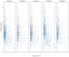 |
Fig. 4. Distribution of the amplitudes and frequencies of (independent) signals not identified as combination frequencies for all 38 SPB stars in our sample, for each of the pre-whitening strategies defined in Table 1. The colour indicates if these signals are involved in a candidate resonance (red) or not (blue), and its gradient indicates the number of detected frequencies: Colours are brighter if more signals are detected within a specific amplitude-frequency bin. The red and blue distributions are plotted independently, so overlap between these distributions is the cause for the appearance of darker, maroon-like coloured bins belonging to the red distribution. The maximal frequency displayed in each panel is 8 d−1, which is the highest frequency of any of the detected (robust two-signal) candidate resonances (see Sect. 4 and, especially, Fig. 10). We display independent signals with an amplitude > 10 ppm because very few independent signals have amplitudes smaller than this limit. |
The effect of a high mode density in the periodogram of KIC005941844 is clearly visible in the bottom panel of Fig. 3: Dozens of small-amplitude signals persist in the residual LS periodogram, which are unresolved with respect to the LD78 criterion. Such unresolved signals can cause modulation of amplitudes and frequencies because they can interfere with other modes (e.g. Bowman et al. 2016) or be residual artefacts from imperfect pre-whitening under the assumption that all oscillations have constant frequencies, amplitudes and phases. In this case the amplitudes of the extracted frequencies are large compared to the amplitudes of these unresolved signals, hence fsv values are not strongly affected by such effects and remain high.
A sometimes neglected point in frequency analysis is that some of the free parameters in the fit to the light curve covary with other free parameters in the fit. Particularly strong covariances exist between the extracted frequencies and their corresponding phases. As an example, neglecting such frequency-phase covariances leads to differences in the frequency values of the two largest-amplitude extracted frequencies of KIC005941844 at the 2σ level when comparing their amplitudes for the same mode frequencies extracted with strategy 5. Covariances among regression parameters not only influence the estimation of relative phases that are crucial to identifying candidate resonances, but can also exert influence on asteroseismic modelling relying on the frequency values (Bowman & Michielsen 2021).
From a purely mathematical point of view, parsimony dictates that any nested regression model that explains the same scaled fraction of variance as a more complex model (i.e. from the same model strategy but containing more free parameters) should be preferred over that more complex model, because of bias-variance trade-off (Claeskens & Hjort 2008). For this reason, one can use information criteria for model selection when the regression models are nested, as per each model strategy separately. However, one cannot use such criteria to distinguish between the capacity of the different regression models based on different stopping criteria and optimisation methods. Moreover, the aim of any asteroseismic data analysis is to deduce as many significant and resolved oscillation frequencies as possible (i.e. we wish to maximise ne as listed in Fig. 1). Since ne is a discrete unknown that we want to maximise, within the adopted conditions on frequency resolution and significance of the modes’ amplitudes, one should not use classical statistical model selection criteria to choose among the strategies 1 to 5. The case of KIC005941844 illustrates this: its five fsv values differ by less than ∼6 × 10⁻³ but the different pre-whitening strategies lead to vastly different ne values. A classical model selection procedure via a BIC or LRT applied to the models based on the different strategies by just using their fsv alone would fail, as it would favour the model obtained by strategy 4 for KIC005941844. However, it is clear that the other four regression models with the vastly larger numbers of extracted modes capture more astrophysical information on, for example, the number of excited modes, potential mode interactions or rotational multiplets. Hence, the aim of finding a good regression model (high fsv) along with a maximum number of resolved oscillation frequencies of significant amplitude (high ne) favour strategies 2, 3, or 5 for this star. These three regression models preferentially select signals at low frequencies, as shown in Fig. 4. The interplay between the physical and (purely) mathematical considerations in selecting the optimal iterative pre-whitening model is challenging. For the SPB stars with high fsv, Fig. 2 shows all five pre-whitening strategies to be almost equivalent by just looking at the summed fsv for the nineteen stars. However, adding the quest to maximise the number of resolved modes gives preference to strategies 2 or 3. In any case, KIC005941844’s large-amplitude oscillations and small-amplitude signals unresolved with respect to the LD78 resolution, as well as its high fsv values, make it a prime target for non-linear asteroseismic analysis.
3.2. Low-fsv stars
High mode densities are observed in the LS periodograms of all low-fsv stars, because dozens of potential signals are left unresolved with respect to the LD78 resolution. Six of the nineteen low-fsv stars furthermore display outburst-like features: marked departures from the baseline brightness of the original light curve, which are in phase with departures from the baseline in the residual light curve. We make a specific distinction between stars that display these features in their light curves and stars that do not. The former are referred to as ‘outbursting stars’, whereas the latter are called ‘high-mode-density stars’. The discussion of the light curve regression model selection for low-fsv stars is therefore guided by examples from both types of low-fsv stars and the overall performance of the regression models in Fig. 2 is split up accordingly.
Oscillation mode density is expected to increase with increasing rotation rate due to rotational frequency shifts. No statistically significant difference is however found between the rotation rates of 26 of the high- and low-fsv stars, derived by Pedersen et al. (2021), as is illustrated by the box plot in Fig. 5. Weighted averages, on the other hand, indicate a difference, as illustrated in Tables 2 and 3. The rotation rate for the high-fsv star we discussed in the previous subsection is located around the centre of the respective class rotation rate distributions, whereas the rotation rates of the low-fsv stars we discuss in this subsection are at the lower boundaries of their distributions (see Tables 2 and 3 for the explicit values). The rotation rate of the high-mode-density star example, KIC008255796, is in fact an outlier in the rotation rate box-and-whisker plot for the low-fsv class, next to the slowly rotating SPB KIC008459899, which is suspected to be a double lined spectroscopic binary due to slightly larger O-C residuals of the fit to its observed spectrum (Lehmann et al. 2011). The latter star is the only (suspected) binary within the pseudo-class of low-fsv stars. Whether and how its binary nature is correlated with its low rotation rate and low fsv is unknown. With the exception of this binary and KIC008255796, the low fsv values of the low-fsv stars thus seem to be connected to rapid rotation.
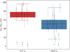 |
Fig. 5. Box-and-whisker plot of the rotation rates of 26 SPB stars obtained from averaging over eight theories of core-boundary and envelope mixing by Pedersen et al. (2021). These are grouped into the two classes defined in this work: low and high fsv, as indicated schematically on the x axis. Whiskers are extended past the quartiles by maximally 1.5 times the interquartile range. Outliers are indicated with a rhombus mark. Individual rotation rates and estimated standard deviations are indicated in grey. The horizontal offset for these rotation rates is imposed for reasons of visibility, without any additional meaning. |
Rotation rates (Ωrot/Ωcrit, Pedersen et al. 2021), highest-fsv pre-whitening strategies, and symbolic largest-amplitude ratio (Aunres/res) for the 19 high-fsv stars, if applicable.
3.2.1. High-mode-density stars
An example of a high-mode-density star, a low-fsv star that does not display outburst-like features in its light curve, is KIC008255796. It was first identified as a misclassified B star by Zhang et al. (2018). Its light curve is shown in the top panel of Fig. 6 and displays periodic variations on longer timescales than KIC005941844, the high-fsv star example. The characteristic properties of the light curves of high-mode-density stars such as KIC008255796 are not dissimilar to those of high-fsv stars. The lower fsv values attained by high-mode-density stars can be attributed to the fact that on average maximal excursions from the baseline brightness are smaller, so that small-amplitude unresolved signals have a larger impact on the fsv value. The maximal excursion from the light curve baseline for KIC005941844 is ∼35 ppt, whereas this value is only ∼6 ppt for KIC008255796, as can be deduced from the top panels of Figs. 3 and 6.
The iteration progress curves of high-mode-density stars are also not dissimilar to those of high-fsv stars, as is illustrated by comparing the middle panels of Figs. 3 and 6, obtained for KIC005941844 and KIC008255796, respectively. The strategy 2 and 3 iteration progress curves of KIC008255796 indicate that more frequencies need to be extracted to reach the ‘optimal model’ for that strategy. This is not unexpected, because these strategies focus their extraction efforts on high-mode-density regions of the periodogram, which are strongly present in the LS periodograms of high-mode-density stars. The other strategies have triggered their stop criteria, and those in which hinting is S/N-based are especially strict, as expected.
The eponymous high mode density within the periodogram is well-illustrated in the bottom panel of Fig. 6 for KIC008255796. Higher mode densities cause more signals to be unresolved with respect to the LD78 criterion, and therefore increase the probability that a larger-amplitude signal is unresolved. Combined with the on average smaller amplitude signals observed in high-mode-density stars compared to high-fsv stars, which are a corollary of the observed differences in maximal excursions from the light curve baseline, a larger influence of unresolved signals on fsv is expected. Indeed, as can be derived from Tables 2 and 3, the average unresolved/resolved amplitude for high-mode-density stars is ∼186/750 ppm, whereas that value is ∼300/5807 ppm for high-fsv stars.
The similarities noted in the light curve and Fourier properties of high-mode-density low-fsv stars and high-fsv stars render their classification somewhat artificial. This is why we refer to the high- and low-fsv stars as pseudo-classes. It is however expected that amplitude modulation (and frequency modulation) more frequently occurs for high-mode-density stars, as they on average exhibit more unresolved signals. Whether that implies that the observed differences in fsv between the two pseudo-classes are not of a purely instrumental origin (i.e. not being able to resolve high mode densities due to limited time span of the photometry), remains to be validated. What is clear, however, is that the amplitude modulation observed in some high-mode-density stars could originate from beating of close frequency pairs (Bowman et al. 2016), or non-linear mode interactions in the intermediate regime (e.g. Buchler et al. 1997; Goupil et al. 1998). Hence, some high-mode-density stars also are prime targets for in-depth non-linear asteroseismic analysis.
3.2.2. Outbursting stars
An example of a low-fsv star that displays the eponymous outburst-like features in its light curve, an outbursting star, is KIC011971405. It was considered to be a prototypical oscillating Be star by Kurtz et al. (2015), and was first identified by McNamara et al. (2012) as an SPB oscillator. Pápics et al. (2017) spectroscopically confirmed it as a Be star, and studied its variability and outbursts in detail. The days-long outburst-like features in its light curve are readily visible in the upper panel of Fig. 7. Similar features can be observed in the light curves of the other outbursting stars, with differing lengths and amplitudes. However, as illustrated in the same panel of Fig. 7, the parts of the light curve of KIC011971405 away from these outburst-like features are very similar to that of a non-outbursting SPB oscillator. This similarity is also noted for the other outbursting stars, and fits within the angular momentum transport model put forward by Neiner et al. (2020) that is used to describe Be star outbursts. Within this model gravito-inertial modes stochastically excited by core convection dominate the LS periodogram at the time of outbursts, whereas g modes excited by the κ mechanism prevail for the entire time span of the light curve. Hence, amplitude and frequency modulation is expected for all outbursting stars, which gives rise to high mode densities in the periodogram. For KIC011971405 modulation has been detected and characterised by Pápics et al. (2017). Interestingly, while for five of six outbursting stars these high mode densities are distinctly grouped, KIC011152422 displays a high mode density in its LS periodogram that spans from 0 to 1 d−1.
The S/N stop criteria trigger an early stop to the pre-whitening (i.e. before 200 frequencies are extracted) for almost all outbursting stars, an example of which can be observed for KIC01197405 in the middle panel of Fig. 7. High mode densities are the main cause for these early triggers. The exception is KIC010285114, whose outburst amplitude, in comparison to the typical excursions from the baseline in its light curve, is the smallest for all outbursting stars. The stop criteria of strategies 4 and 5 trigger early abortion of the pre-whitening for all outbursting stars, whereas the iteration progress curves for strategies 2 and 3 indicate more frequencies can be extracted.
The high mode densities in the LS periodograms and the outburst-like features in the light curves are also the prime factors to which the low fsv values for outbursting stars can be attributed. Because of these high mode densities we do not expect any significant changes in fsv after incorporating additional frequencies extracted by strategies 2 and 3 for KIC01197405, and the other outbursting stars. The observed amplitude modulation and outbursts in the outbursting stars in our sample could also be linked to many g modes coming into phase with each other, some of which by non-linear interaction (Kurtz et al. 2015). If this is the sole origin of the outbursts, it corroborates the idea that oscillating Be stars are complex analogues of SPB stars (Aerts 2006), and supports the idea of the artificiality of the high- and low-fsv pseudo-classes that was discussed in the previous subsection. The Kurtz et al. (2015) theory relies upon a light curve model similar to the one utilised in this work, consisting of (interacting) sinusoids of constant amplitude and frequency. Kurtz et al. (2015) show that the bulk of the variability of KIC011971405 can be modelled in such a manner. Whether such a light curve model is sufficient to explain the bulk of the observed modulation for all of the outbursting B stars observed by Kepler remains to be verified, but this is outside of the scope of this work. As seen from Figs. 1 and 2, the choice in pre-whitening strategy clearly exerts a stronger influence for outbursting stars than for the other SPB stars.
4. Results: Candidate resonance characteristics
We now discuss the results of our search for candidate non-linear g-mode resonances within the light curve models obtained for the pre-whitening strategies applied to all stars in our sample. The degree to which non-linear interactions are important increases with pulsation amplitude. We therefore limit our search for candidate resonances to the combination frequencies that include as a parent frequency at least one of the two largest-amplitude oscillation signals detected in the light curves, or both. We hereafter refer to such candidate resonances as ‘two-signal’ candidate resonances. We also verify whether the number of two-signal candidate resonances is correlated to the binary or outbursting nature of the SPB stars, or their fsv-based pseudo-classification. More candidate resonances that do not involve these two largest-amplitude signals may be detectable. We discuss these additional candidate resonances for each star in the sample in Appendix B, in which we also indicate the priority for non-linear asteroseismic follow-up.
The strategy discussed in Sect. 2.3 is employed to identify two-signal candidate resonances in the frequency-locked regime of mode interaction for the models generated by all five strategies for each star. To do so, we verify whether the highest-fsv strategy that performs non-linear least-squares optimisation of the frequencies (i.e. one of strategies 1−4) contains unique matches in frequency to within 1 Rayleigh limit at the 1σ level, with the frequencies in the linear regression model generated by pre-whitening strategy 5:

In Eq. (9) νfsv denotes the frequency of the model that attains the highest-fsv among all strategies that employ non-linear least-squares optimisation, and νlin denotes the frequency obtained for pre-whitening strategy 5. We refer to candidate resonances for which Eq. (9) is fulfilled as ‘robust’ candidate resonances and discuss how their occurrence co-varies with pseudo-classification in Sect. 4.1. We also discuss how this is reflected in the characteristic properties of these resonances in Sect. 4.2.
Baran et al. (2015) and Zong et al. (2016a) note that the Breger et al. (1993) S/N detection threshold of 4.0 is low as a detection threshold for signals in K2 data and Kepler short-cadence data, respectively. On the other hand, Degroote et al. (2009a,b) concluded that not all signals failing the Breger et al. (1993) threshold correspond to noise peaks (i.e. S/N-based methods are not clearcut in their optimal cut-off value as significance criterion). We therefore make an additional distinction between frequencies with S/N ≥ 5 and S/N < 5 for the detection and analysis of candidate resonances in the following subsections.
4.1. Numbers of identified candidate resonances
The numbers of two-signal candidate resonances, with an indication of how many of those candidate resonances have S/N values ≥5, are displayed in Table 4 for all five strategies applied to each star in our sample. The number of robust two-signal candidate resonances and its S/N ≥ 5 counterpart are also shown. It is apparent that for every star in our sample there is at least one pre-whitening strategy that delivers a final light curve model in which two-signal candidate resonances are identified. For 32 out of 38 stars (∼84%) we find robust resonance identifications using the definition in Eq. (9). Imposing the additional S/N ≥ 5 restriction lowers this number to 24 out of 38 stars (∼63%). More candidate resonances are identified if we loosen the restriction on involvement of the two largest-amplitude candidate resonances. Candidate resonances are thus omnipresent in the light curves of the SPB stars we consider in this work, and SPB stars in general are therefore intrinsic non-linear non-radial oscillators.
Number of two-signal candidate resonances for each of the five pre-whitening strategies applied to all stars in our sample, and the number of two-signal candidate resonances defined as ‘robust’.
The covariance matrices of the light curve models obtained from applying the pre-whitening strategies to all stars in the sample vary from strategy to strategy and from star to star. The figures of Appendix A display visualisations of the covariance matrices obtained for the highest-fsv pre-whitening strategy (i.e. the best regression model), in a block-normalised form, which is discussed in detail in Appendix A.4. An example of such a visualisation of a covariance matrix is given in Fig. 8, which displays the covariance matrix of the best regression model of the light curve of the high-fsv star KIC005941844. Large numbers of weak inter-parameter covariations and the strong frequency-phase covariations mentioned in Sect. 3.1 can be seen, similar to what is observed in all covariance matrices displayed in Appendix A.4. These covariations differ from star to star. Several covariance and correlation matrices display a structured pattern within their different blocks (i.e. they are structured) that indicates the strongest inter-parameter covariations and correlations.
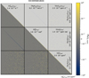 |
Fig. 8. Covariance matrix of the best regression model of the light curve of KIC005914844 (obtained from pre-whitening strategy 3) in the block-normalised form described in Appendix A.4 and Fig. A.1. The colour map shows the normalised (co)variance values (SN)ij, norm, and the change in darkness between the upper and lower triangular part of the matrix is only for visualisation purposes. |
The covariance matrix propagates into the relative frequencies and phases defined in Eqs. (4) and (5), which are used to identify a candidate resonance. The occurrence of robust candidate resonances as indicated in Table 4 thus connects to the covariance matrix structure among differing light curve models.
In asteroseismic forward modelling one compares observed mode frequencies with frequencies obtained from models of stellar evolution. As Davies et al. (2016) note for asteroseismic modelling based on solar-like oscillations, it is essential to account for regression parameter covariances and correlations in this process. Regression parameter covariances and correlations can also impact asteroseismic forward modelling based on gravity modes, as discussed in Sect. 3.1. These covariances and correlations also impact non-linear asteroseismic modelling, which utilises extracted amplitudes, phases, and derived quantities such as the frequency de-tuning δν and the relative phase Φ, next to the extracted frequencies. The strong frequency-phase covariances detected in all covariance matrices displayed in Appendix A.4 therefore render it necessary to include such correlations and covariances in future non-linear asteroseismic modelling of the SPB stars in our sample.
No differences in the number of identified two-signal candidate resonances are found when comparing the models of stars belonging to the low- and high-fsv pseudo-classes, as is shown in the left panel of Fig. 9. This conclusion is not changed when only considering two-signal candidate resonances with S/N ≥ 5. The box-and-whisker plots in that panel furthermore show that no significant dependence on pre-whitening strategy can be identified. Any additional uncertainty in parameter values due to covariance among parameters is neglected in the construction of the box-and-whisker plots. However, including such uncertainties in their construction would only support the conclusion that no significant dependences are observed.
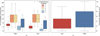 |
Fig. 9. Box-and-whisker plots of the number of identified two-signal candidate resonances or the number of identified robust two-signal candidate resonances (defined by Eq. (9)), grouped by the pseudo-classes defined in this work: low and high fsv. Left panel: box-and-whisker plot of the number of identified two-signal candidate resonances. The colour depicts the pre-whitening strategy employed to generate the light curve models. Right panel: box-and-whisker plot of the number of identified robust two-signal candidate resonances. Whiskers and outliers for both panels are indicated in a similar way to how they are indicated in Fig. 5. |
One might suspect that the differing (rich) objective function landscape for which the global minimum is sought during optimisation is a reason for a difference between stars belonging to the two pseudo-classes, high and low fsv. Amplitude modulation is more important in shaping this landscape for low-fsv stars than for their high-fsv counterparts, although this varies from star to star and from signal to signal. However, no difference in number of identified two-signal robust candidate resonances (i.e. those that fulfil the condition in Eq. (9)) can be noted when comparing the two pseudo-classes, as is shown on the right panel of Fig. 9. This lack of difference is also noted for robust two-signal candidate resonances with S/N ≥ 5. Besides a few exceptions, amplitude modulation of low-fsv star signals thus seems to have only a minor influence on the identification of signals relevant for (two-signal) robust candidate resonances.
We find no evidence for a distinction in number of identified candidate resonances when comparing the numbers strategy per strategy for outbursting and non-outbursting stars, even if we only compare candidate resonances for which S/N ≥ 5. A class imbalance exists when making the latter comparison (8 outbursting stars vs. 30 non-outbursting stars). However, the presence of robust candidate resonances in stars of all (pseudo-)classes supports the lack of distinction between outbursting and non-outbursting stars. It also lends support to the interpretation of Be star variability in which the times of outbursts signify several modes coming into phase (e.g. Kurtz et al. 2015).
Finally, we also check for correlation of the number of candidate resonances with binarity. Two stars in our sample are confirmed binaries, KIC006352430 (Pápics et al. 2013) and KIC004930889 (Pápics et al. 2017), whereas Lehmann et al. (2011) suspect KIC008459899 to be a binary as well. All other stars in our sample do not have confirmed or suspected binary companions. We find no difference in the number of identified two-signal candidate resonances between (suspected) binary and single SPB stars, and only including candidate resonances for which S/N ≥ 5 does not make a difference.
4.2. Characteristic properties of identified candidate resonances
Amplitudes, frequencies, frequency de-tunings δν, relative amplitudes Ar, and relative phases Φ define candidate resonances. These characteristic properties were for example discussed by Degroote et al. (2009a) for a β Cep (CoRoT) star, HD 180642, whereas Vuille (2000) and Vuille & Brassard (2000) discussed them for an oscillating DA white dwarf, G29-38. We present how these properties covary in Fig. 10 for the identified robust two-signal candidate resonances of all stars in our sample. The amplitudes and frequencies of signals involved in these resonances are not significantly different from those not involved in them, as shown in Fig. 4.
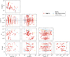 |
Fig. 10. Highest-fsv strategy characteristic properties of the identified robust candidate resonances, which involve the two largest-amplitude signals, as a function of each other, with 1σ uncertainties indicated: amplitude A, frequency ω/2π, frequency de-tuning δν (see Eq. (4)), relative phase Φ (see Eq. (5)), and relative amplitude Ar (see Eq. (6)). Colours indicate the different pseudo-classes to which the stars that exhibit the candidate resonances belong. The transparent symbols indicate robust candidate resonances having 4 < S/N < 5, whereas the full symbols indicate robust candidate resonances for which S/N ≥ 5. Grey lines indicate the zero point for the frequency de-tuning, and the faint grey horizontal lines in the last row of panels indicate the relative phases that satisfy Eq. (5). |
Most robust (two-signal) candidate resonances originate from high fsv stars, as can be seen in Table 4. The panels in the left column of Fig. 10 show that most robust two-signal candidate resonances exhibit frequencies ≲2.5 d−1. Several of those low-frequency (ω/2π ≲ 2.5 d−1) candidate resonances have 4 < S/N < 5. The bulk of the high-frequency robust two-signal candidate resonances (ω/2π ≳ 2.5 d−1) depicted in the top panel of Fig. 10 exhibit amplitudes < 100 ppm, whereas the bulk of the low-frequency robust two-signal candidate resonances exhibit amplitudes varying from ∼30 to ∼300 ppm. Only a few of the detected robust two-signal candidate resonances have amplitudes ≥200 ppm, predominantly at low frequencies. Similarly, only a few robust two-signal candidate resonances are detected with amplitudes of the order of 10 ppm. Few of the frequency de-tunings of the robust candidate resonances are significantly different from 0 d−1, as can be deduced from the panels in Fig. 10 that display the frequency de-tunings (δν). This is expected because of the way we selected robust candidate resonances (see Eq. (9)). The few outliers we observe likely belong to either the frequency-locked regime or the intermediate regime, although definitive conclusions can only be made if the linear growth rate γ of the mode is known, which requires non-linear asteroseismic models. No distinct trends are present in any of the panels of Fig. 10 that display the relative phases (Φ) and the relative amplitudes (Ar).
Variances for the characteristic properties are larger than average for robust two-signal candidate resonances that have extreme amplitudes. By comparing the individual properties of the two-signal candidate resonances for each star in our sample, we find that the largest-amplitude signals shown in Fig. 10 are the robust two-signal candidate resonances of KIC009715425 and KIC010526294. The larger uncertainties in their properties are attributable to the high mode density for the outbursting star KIC009715425, and the unresolved rotationally split triplet signals in the light curve of KIC010526294 (Pápics et al. 2014). The covariance matrices of the best light curve regression models of these stars are strongly structured, as shown in Figs. A.6 and A.7, indicating significant covariance among some of the regression parameters. For the small-amplitude signals shown in Fig. 10, the increased variance of the characteristic properties is explained by the fact that the signals are closer to the noise level, as is indicated by half of these signals having 4 < S/N < 5.
The approach taken in this section to characterise candidate resonances contains the conservative approximation of cataloguing only the candidate resonances influenced by the two largest-amplitude signals. It is thus limited in capturing the characteristic properties of candidate resonances. This raises questions that need to be solved, including (i) whether the conservative approach that only considers robust candidate resonances defined by Eq. (9) is satisfactory for initial target selection for non-linear asteroseismic studies; (ii) assuming the conservative approach is satisfactory, how the number and characteristic properties of candidate resonances change if more, lower-amplitude signals are allowed to be involved in the candidate resonances; and (iii) whether it is expected from non-linear stellar oscillation theory that no significant trends exist among the characteristic candidate resonance properties.
The second question is dealt with in Appendix B, whereas the other questions require non-linear asteroseismic models in order to be answered, which we plan to take up in follow-up studies.
5. Conclusions and prospects
We analysed the Kepler light curves of an ensemble of 38 SPB stars by making use of five different iterative pre-whitening strategies. Amplitude-based pre-whitening strategies tend to extract larger-amplitude signals from the lower-frequency, mode-dense regions of the LS periodograms in g-mode pulsators, whereas S/N-based pre-whitening strategies tend to extract more smaller-amplitude signals at higher-frequency, mode-scarce regions, as illustrated in Fig. 4.
The scaled fraction of variance fsv, defined in Eq. (3), is one of the metrics used to compare the frequency analysis results in order to select the optimal model for the light curve. Based on that metric, as well as the (residual) LS periodogram and light curve, we divide the stars in our sample into three different pseudo-classes: the high-fsv, the high-mode-density, and the outbursting pseudo-classes. The first pseudo-class consists of 19 stars for which the models of all five pre-whitening strategies attain fsv values > 0.9. The two other pseudo-classes are discerned by the detection of outburst-like features. We refer to them as pseudo-classes because we found that some of their characterising properties are attributable to the limited frequency resolution, which does not allow one to resolve several of the signals observed in the Kepler light curves. This limited frequency resolution can be attributed to the high mode densities that are detected in the LS periodograms, which also leads to modulation of some of the detected signals. The resonant excitation of envelope g modes with inertial modes propagating in the core, which requires rapid rotation to be efficient (Lee 2021), may also be a reason why SPB stars exhibit such mode-dense LS periodograms.
An important point in the frequency analysis of SPB stars is the covariance among the fitting parameters. We demonstrate the particularly strong covariances between extracted frequencies and phases in the figures in Appendix A. These covariances are sometimes neglected in the uncertainty budget of the light curve models such that regression parameter uncertainties are underestimated. It is necessary to include such regression parameter covariations in future asteroseismic modelling of the SPB stars in our sample.
The role of resonances among g modes was described eloquently by Buchler et al. (1997). Few to no space-based photometric data were available at the time to match the mainly theoretical discussions of its importance. Lee (2012) provided an account of the importance of rotation on non-linear mode interactions in the rapidly rotating B stars by studying g modes excited in stellar models near the zero-age MS. Applications of this theory were limited by the lack of available photometric data. Because we now have the full Kepler dataset at our disposal, the research field of non-linear asteroseismology applied to MS g-mode pulsators can be reinvigorated. Although intermediate-mass dwarfs have primarily been the target of linear asteroseismic studies for widely differing purposes, such as their sizing, weighing, ageing (Serenelli et al. 2021), and the characterisation of their internal rotation and mixing (e.g. Pedersen et al. 2021; Michielsen et al. 2021), no observation-based modelling studies have focused on non-linear mode interactions.
Given the observed deficit of angular momentum transport during the MS in current stellar evolution models (Aerts et al. 2019), the importance of non-linear mode interactions for angular momentum transport deserves follow-up studies. In this work we provide an observational basis for this. Based on the light curve models constructed during frequency analysis, we identified second-order candidate direct resonant Kepler SPB oscillations. We guided ourselves in this identification process using the frequency de-tuning and relative phase relations defined in Eqs. (4) and (5), inspired by Van Hoolst (1995) and Buchler et al. (1997). Future non-linear asteroseismic models describing frequency-locked signals based on the AEs will make use of such characteristic properties of candidate resonances (as well as the relative amplitude defined in Eq. (6)), or properties derived therefrom.
It is more likely that a resonant g-mode interaction occurs if one of the parent frequencies has a large amplitude. As a first approximation we look at the number of identified candidate resonances that involve the two largest-amplitude signals in the light curve, which we refer to as two-signal candidate resonances, and the characteristic properties of such resonances. We find that 32 of the 38 SPB stars turn out to be intrinsic non-linear g-mode oscillators, reiterating the need for the quantification of the non-linear g-mode interactions.
One should take into account that the practical implementation of the criterion indicating that the frequency de-tuning relation is fulfilled is only approximate, because the growth rates needed to verify the Buchler et al. (1997) criterion cannot be derived directly from observations. Moreover, as Goupil et al. (1998) explained, the boundaries of the Buchler et al. (1997) regimes of resonant mode interaction might not be that distinct for observational data, and they are undetermined for SPB stars. A step towards the determination of the Buchler et al. (1997) regimes consists in verifying whether the candidate resonances detected in this work display the oscillatory behaviour that is deemed characteristic of the intermediate regime (Goupil et al. 1998). This is a next logical step in characterising g-mode resonances in SPB stars.
Our current observational analyses constitute the ground work for performing forward asteroseismic modelling of the non-linear mode properties, with the aim to investigate whether it leads to different or additional results on internal rotation and mixing compared to what is derived from the current (linear) state-of-the-art approach to asteroseismic modelling of SPB stars (Pedersen et al. 2021).
Acknowledgments
The research leading to these results received funding from the European Research Council (ERC) under the European Union’s Horizon 2020 research and innovation program (grant agreement No. 670519: MAMSIE with PI CA.), and from the KU Leuven Research Council (grant C16/18/005: PARADISE, with PI CA.). DMB is grateful for a senior post-doctoral fellowship from the Research Foundation Flanders (FWO) with grant agreement No. 1286521N. TVR gratefully acknowledges support from the Research Foundation Flanders (FWO) under grant agreement nr. 12ZB620N. This research was supported in part by the National Science Foundation under Grant No. NSF PHY-1748958. A part of the computational resources and services used in this work were provided by the VSC (Flemish Supercomputer Center), funded by the Research Foundation – Flanders (FWO) and the Flemish Government – department EWI. We thank the anonymous referee and the language editor, R. Baier, for the useful comments on the manuscript. JVB thanks J. De Ridder for his advice on visualising correlations among light curve regression model parameters, and thanks W. Zong for his useful comments on the manuscript. Throughout this work we have made use of the following Python packages: LMFIT (Newville et al. 2020), SCIPY (Virtanen et al. 2020), NUMPY (Harris et al. 2020), PANDAS (McKinney 2010), MATPLOTLIB (Hunter 2007), and SEABORN (Waskom & the Seaborn Development Team 2020). We thank their authors for making these great software packages open source.
References
- Aerts, C. 2006, in Proceedings of SOHO 18/GONG 2006/HELAS I, Beyond the spherical Sun, eds. K. Fletcher, & M. Thompson, ESA Spec. Publ., 624, 131 [NASA ADS] [Google Scholar]
- Aerts, C., De Cat, P., Peeters, E., et al. 1999, A&A, 343, 872 [NASA ADS] [Google Scholar]
- Aerts, C., Christensen-Dalsgaard, J., & Kurtz, D. W. 2010, Asteroseismology, Astronomy and Astrophysics Library (Netherlands: Springer) [Google Scholar]
- Aerts, C., Van Reeth, T., & Tkachenko, A. 2017, ApJ, 847, L7 [Google Scholar]
- Aerts, C., Mathis, S., & Rogers, T. M. 2019, ARA&A, 57, 35 [Google Scholar]
- Auvergne, M., Bodin, P., Boisnard, L., et al. 2009, A&A, 506, 411 [NASA ADS] [CrossRef] [EDP Sciences] [Google Scholar]
- Balona, L. A., Pigulski, A., De Cat, P., et al. 2011, MNRAS, 413, 2403 [Google Scholar]
- Balona, L. A., Baran, A. S., Daszyńska-Daszkiewicz, J., & De Cat, P. 2015, MNRAS, 451, 1445 [Google Scholar]
- Baran, A. S., Koen, C., & Pokrzywka, B. 2015, MNRAS, 448, L16 [NASA ADS] [CrossRef] [Google Scholar]
- Barceló Forteza, S., Michel, E., Roca Cortés, T., & García, R. A. 2015, A&A, 579, A133 [NASA ADS] [CrossRef] [EDP Sciences] [Google Scholar]
- Borucki, W. J., Koch, D., Basri, G., et al. 2010, Science, 327, 977 [Google Scholar]
- Bouabid, M. P., Dupret, M. A., Salmon, S., et al. 2013, MNRAS, 429, 2500 [Google Scholar]
- Bowman, D. M., & Kurtz, D. W. 2014, MNRAS, 444, 1909 [NASA ADS] [CrossRef] [Google Scholar]
- Bowman, D. M., & Michielsen, M. 2021, A&A, in press, https://doi.org/10.1051/0004-6361/202141726 [Google Scholar]
- Bowman, D. M., Kurtz, D. W., Breger, M., Murphy, S. J., & Holdsworth, D. L. 2016, MNRAS, 460, 1970 [NASA ADS] [CrossRef] [Google Scholar]
- Bowman, D. M., Hermans, J., Daszyńska-Daszkiewicz, J., et al. 2021, MNRAS, 504, 4039 [NASA ADS] [CrossRef] [Google Scholar]
- Breger, M., Stich, J., Garrido, R., et al. 1993, A&A, 271, 482 [NASA ADS] [Google Scholar]
- Buchler, J. R. 1993, Ap&SS, 210, 9 [NASA ADS] [CrossRef] [Google Scholar]
- Buchler, J. R., & Goupil, M. J. 1984, ApJ, 279, 394 [CrossRef] [Google Scholar]
- Buchler, J. R., Goupil, M. J., & Hansen, C. J. 1997, A&A, 321, 159 [NASA ADS] [Google Scholar]
- Buysschaert, B., Aerts, C., Bowman, D. M., et al. 2018, A&A, 616, A148 [NASA ADS] [CrossRef] [EDP Sciences] [Google Scholar]
- Christophe, S., Ballot, J., Ouazzani, R. M., Antoci, V., & Salmon, S. J. A. J. 2018, A&A, 618, A47 [NASA ADS] [CrossRef] [EDP Sciences] [Google Scholar]
- Claeskens, G., & Hjort, N. L. 2008, Model Selection and Model Averaging, Cambridge Series in Statistical and Probabilistic Mathematics (Cambridge: Cambridge University Press) [Google Scholar]
- Davies, G. R., Silva Aguirre, V., Bedding, T. R., et al. 2016, MNRAS, 456, 2183 [Google Scholar]
- Debosscher, J., Blomme, J., Aerts, C., & De Ridder, J. 2011, A&A, 529, A89 [NASA ADS] [CrossRef] [EDP Sciences] [Google Scholar]
- De Cat, P., & Aerts, C. 2002, A&A, 393, 965 [NASA ADS] [CrossRef] [EDP Sciences] [Google Scholar]
- De Cat, P., Aerts, C., De Ridder, J., et al. 2000, A&A, 355, 1015 [NASA ADS] [Google Scholar]
- De Cat, P., Briquet, M., Daszyńska-Daszkiewicz, J., et al. 2005, A&A, 432, 1013 [NASA ADS] [CrossRef] [EDP Sciences] [Google Scholar]
- De Cat, P., Briquet, M., Aerts, C., et al. 2007, A&A, 463, 243 [NASA ADS] [CrossRef] [EDP Sciences] [Google Scholar]
- Degroote, P., Briquet, M., Catala, C., et al. 2009a, A&A, 506, 111 [NASA ADS] [CrossRef] [EDP Sciences] [Google Scholar]
- Degroote, P., Aerts, C., Ollivier, M., et al. 2009b, A&A, 506, 471 [NASA ADS] [CrossRef] [EDP Sciences] [Google Scholar]
- Degroote, P., Aerts, C., Baglin, A., et al. 2010, Nature, 464, 259 [Google Scholar]
- Dhouib, H., Prat, V., Van Reeth, T., & Mathis, S. 2021, A&A, 652, A154 [NASA ADS] [CrossRef] [EDP Sciences] [Google Scholar]
- Dziembowski, W. 1982, Acta Astron., 32, 147 [NASA ADS] [Google Scholar]
- Dziembowski, W., & Krolikowska, M. 1985, Acta Astron., 35, 5 [NASA ADS] [Google Scholar]
- Dziembowski, W. A., Moskalik, P., & Pamyatnykh, A. A. 1993, MNRAS, 265, 588 [NASA ADS] [Google Scholar]
- Gautschy, A., & Saio, H. 1993, MNRAS, 262, 213 [NASA ADS] [CrossRef] [Google Scholar]
- Goupil, M. J., Dziembowski, W. A., & Fontaine, G. 1998, Balt. Astron., 7, 21 [NASA ADS] [Google Scholar]
- Harris, C. R., Millman, K. J., van der Walt, S. J., et al. 2020, Nature, 585, 357 [NASA ADS] [CrossRef] [Google Scholar]
- Henneco, J., Van Reeth, T., Prat, V., et al. 2021, A&A, 648, A97 [EDP Sciences] [Google Scholar]
- Hunter, J. D. 2007, Comput. Sci. Eng., 9, 90 [NASA ADS] [CrossRef] [Google Scholar]
- James, F. 1994, MINUIT Function Minimization and Error Analysis: Reference Manual Version 94.1, CERN-D-506, CERN-D506 [Google Scholar]
- Kurtz, D. W., Shibahashi, H., Murphy, S. J., Bedding, T. R., & Bowman, D. M. 2015, MNRAS, 450, 3015 [NASA ADS] [CrossRef] [Google Scholar]
- Lee, U. 2012, MNRAS, 420, 2387 [NASA ADS] [CrossRef] [Google Scholar]
- Lee, U. 2021, MNRAS, 505, 1495 [NASA ADS] [CrossRef] [Google Scholar]
- Lee, U., & Saio, H. 1997, ApJ, 491, 839 [Google Scholar]
- Lehmann, H., Tkachenko, A., Semaan, T., et al. 2011, A&A, 526, A124 [NASA ADS] [CrossRef] [EDP Sciences] [Google Scholar]
- Lomb, N. R. 1976, Ap&SS, 39, 447 [Google Scholar]
- Longuet-Higgins, M. S. 1968, Phil. Trans. R. Soc. London Ser. A, 262, 511 [CrossRef] [Google Scholar]
- Loumos, G. L., & Deeming, T. J. 1978, Ap&SS, 56, 285 [CrossRef] [Google Scholar]
- Mathias, P., Aerts, C., Briquet, M., et al. 2001, A&A, 379, 905 [NASA ADS] [CrossRef] [EDP Sciences] [Google Scholar]
- Mathis, S. 2013, in Transport Processes in Stellar Interiors, eds. M. Goupil, K. Belkacem, C. Neiner, F. Lignières, & J. J. Green, 865, 23 [Google Scholar]
- Mathis, S., & Prat, V. 2019, A&A, 631, A26 [NASA ADS] [CrossRef] [EDP Sciences] [Google Scholar]
- McKinney, W. 2010, in Proceedings of the 9th Python in Science Conference, eds. S. van der Walt, & J. Millman, 56 [Google Scholar]
- McNamara, B. J., Jackiewicz, J., & McKeever, J. 2012, AJ, 143, 101 [NASA ADS] [CrossRef] [Google Scholar]
- Michielsen, M., Aerts, C., & Bowman, D. M. 2021, A&A, 650, A175 [NASA ADS] [CrossRef] [EDP Sciences] [Google Scholar]
- Miglio, A., Montalbán, J., Noels, A., & Eggenberger, P. 2008, MNRAS, 386, 1487 [Google Scholar]
- Montgomery, M. H., & O’Donoghue, D. 1999, Delta Scuti Star Newsletter, 13, 28 [NASA ADS] [Google Scholar]
- Moravveji, E., Aerts, C., Pápics, P. I., Triana, S. A., & Vandoren, B. 2015, A&A, 580, A27 [NASA ADS] [CrossRef] [EDP Sciences] [Google Scholar]
- Moravveji, E., Townsend, R. H. D., Aerts, C., & Mathis, S. 2016, ApJ, 823, 130 [NASA ADS] [CrossRef] [Google Scholar]
- More, J. J., Garbow, B. S., & Hillstrom, K. E. 1980, User guide for MINPACK-1. [In FORTRAN] [CrossRef] [Google Scholar]
- Neiner, C., Lee, U., Mathis, S., et al. 2020, A&A, 644, A9 [EDP Sciences] [Google Scholar]
- Newville, M., Otten, R., Nelson, A., et al. 2020, https://doi.org/10.5281/zenodo.3814709 [Google Scholar]
- Oliphant, T. E. 2006, A Bayesian Perspective on Estimating Mean, Variance, and Standard-deviation from Data [Google Scholar]
- Ouazzani, R. M., Lignières, F., Dupret, M. A., et al. 2020, A&A, 640, A49 [NASA ADS] [CrossRef] [EDP Sciences] [Google Scholar]
- Pamyatnykh, A. A. 1999, Acta Astron., 49, 119 [Google Scholar]
- Pápics, P. I. 2012, Astron. Nachr., 333, 1053 [CrossRef] [Google Scholar]
- Pápics, P. I., Briquet, M., Baglin, A., et al. 2012, A&A, 542, A55 [NASA ADS] [CrossRef] [EDP Sciences] [Google Scholar]
- Pápics, P. I., Tkachenko, A., Aerts, C., et al. 2013, A&A, 553, A127 [NASA ADS] [CrossRef] [EDP Sciences] [Google Scholar]
- Pápics, P. I., Moravveji, E., Aerts, C., et al. 2014, A&A, 570, A8 [NASA ADS] [CrossRef] [EDP Sciences] [Google Scholar]
- Pápics, P. I., Tkachenko, A., Aerts, C., et al. 2015, ApJ, 803, L25 [Google Scholar]
- Pápics, P. I., Tkachenko, A., Van Reeth, T., et al. 2017, A&A, 598, A74 [Google Scholar]
- Pedersen, M. G. 2020, PhD Thesis, KU Leuven, Belgium [Google Scholar]
- Pedersen, M. G., Aerts, C., Pápics, P. I., et al. 2021, Nat. Astron., 5, 715 [NASA ADS] [CrossRef] [Google Scholar]
- Prat, V., Mathis, S., Buysschaert, B., et al. 2019, A&A, 627, A64 [NASA ADS] [CrossRef] [EDP Sciences] [Google Scholar]
- Prat, V., Mathis, S., Neiner, C., et al. 2020, A&A, 636, A100 [NASA ADS] [CrossRef] [EDP Sciences] [Google Scholar]
- Press, W. H., Teukolsky, S. A., Vetterling, W. T., et al. 2007, Numerical Recipes 3rd Edition: The Art of Scientific Computing (Cambridge: Cambridge University Press) [Google Scholar]
- Rivinius, T., Carciofi, A. C., & Martayan, C. 2013, A&ARv, 21, 69 [Google Scholar]
- Rivinius, T., Baade, D., & Carciofi, A. C. 2016, A&A, 593, A106 [NASA ADS] [CrossRef] [EDP Sciences] [Google Scholar]
- Saio, H., Takata, M., Lee, U., Li, G., & Van Reeth, T. 2021, MNRAS, 502, 5856 [Google Scholar]
- Scargle, J. D. 1982, ApJ, 263, 835 [Google Scholar]
- Schwarzenberg-Czerny, A. 1991, MNRAS, 253, 198 [CrossRef] [Google Scholar]
- Schwarzenberg-Czerny, A. 2003, in Interplay of Periodic, Cyclic and Stochastic Variability in Selected Areas of the H-R Diagram, ed. C. Sterken, ASP Conf. Ser., 292, 383 [NASA ADS] [Google Scholar]
- Serenelli, A., Weiss, A., Aerts, C., et al. 2021, A&ARv, 29, 4 [Google Scholar]
- Simon, N. R., & Lee, A. S. 1981, ApJ, 248, 291 [NASA ADS] [CrossRef] [Google Scholar]
- Szewczuk, W., & Daszyńska-Daszkiewicz, J. 2018, MNRAS, 478, 2243 [Google Scholar]
- Szewczuk, W., Walczak, P., & Daszyńska-Daszkiewicz, J. 2021, MNRAS, 503, 5894 [NASA ADS] [CrossRef] [Google Scholar]
- Townsend, R. H. D. 2003, MNRAS, 340, 1020 [Google Scholar]
- Triana, S. A., Moravveji, E., Pápics, P. I., et al. 2015, ApJ, 810, 16 [Google Scholar]
- Van Beeck, J., Prat, V., Van Reeth, T., et al. 2020, A&A, 638, A149 [NASA ADS] [CrossRef] [EDP Sciences] [Google Scholar]
- Van Hoolst, T. 1994a, A&A, 292, 471 [NASA ADS] [Google Scholar]
- Van Hoolst, T. 1994b, A&A, 286, 879 [NASA ADS] [Google Scholar]
- Van Hoolst, T. 1995, A&A, 295, 371 [Google Scholar]
- Van Hoolst, T. 1996, A&A, 308, 66 [NASA ADS] [Google Scholar]
- Van Hoolst, T., & Smeyers, P. 1993, A&A, 279, 417 [NASA ADS] [Google Scholar]
- Virtanen, P., Gommers, R., Oliphant, T. E., et al. 2020, Nat. Meth., 17, 261 [Google Scholar]
- Vuille, F. 2000, MNRAS, 313, 179 [NASA ADS] [CrossRef] [Google Scholar]
- Vuille, F., & Brassard, P. 2000, MNRAS, 313, 185 [NASA ADS] [CrossRef] [Google Scholar]
- Waelkens, C. 1991, A&A, 246, 453 [NASA ADS] [Google Scholar]
- Waelkens, C., & Rufener, F. 1985, A&A, 152, 6 [NASA ADS] [Google Scholar]
- Waskom, M., & the Seaborn Development Team 2020, https://doi.org/10.5281/zenodo.592845 [Google Scholar]
- Wu, Y. 2001, MNRAS, 323, 248 [NASA ADS] [CrossRef] [Google Scholar]
- Zhang, C., Liu, C., Wu, Y., et al. 2018, ApJ, 854, 168 [Google Scholar]
- Zong, W., Charpinet, S., Vauclair, G., Giammichele, N., & Van Grootel, V. 2016a, A&A, 585, A22 [NASA ADS] [CrossRef] [EDP Sciences] [Google Scholar]
- Zong, W., Charpinet, S., & Vauclair, G. 2016b, A&A, 594, A46 [NASA ADS] [CrossRef] [EDP Sciences] [Google Scholar]
Appendix A: LMFIT configuration and covariance estimation
This appendix contains detailed information on the configuration of the LMFIT python package (Newville et al. 2020) that is employed for the least-squares optimisations. We discuss the optimisation methods employed in this work and their configurational parameters separately, in Sects. A.1 and A.2. The third subsection, A.3, discusses how bounds are enforced on the optimisation parameters for the optimisation method discussed in Sect. A.1. A fourth subsection, A.4, discusses the covariance and correlation matrices of the regression models.
A.1. LMFIT Levenberg-Marquardt method
The LMFIT Levenberg-Marquardt method (‘leastsq’) is employed in this work to obtain the final optimised parameters in each iterative pre-whitening step, using the parameter hints as initial values. This optimisation method makes use of the SCIPY leastsq method (Virtanen et al. 2020), which itself uses the MINPACK-1 lmdif and lmder sum-of-squares minimisation algorithms (More et al. 1980). In this work, the Jacobian matrix was estimated by its forward-difference approximation implemented in the MINPACK-1 lmdif algorithm.
Three separate convergence tests were conducted, each of which has its own convergence parameter. The xtol parameter indicates the desired relative error in the approximate solution between two consecutive iterates. The ftol parameter measures the desired relative error in the sum of squares, and the gtol parameter indicates the desired orthogonality between the evaluated result (the function vector) and the columns of the computed Jacobian matrix. The convergence parameters xtol, ftol and gtol were all set to 10−7. More information on the conducted convergence tests can be found in the MINPACK-1 documentation (More et al. 1980). The maximum number of function evaluations was set to 2000(npv + 1), where npv is the number of variable parameters in the regression model.
Because the MINPACK-1 implementation does not support hard constraints on regression parameters, the LMFIT implementation feeds transformed internal variables (that enforce the bounds) to the SCIPY/MINPACK-1 solver. These variables are back-transformed after the optimisation (including a rescaling of the Jacobian matrix) to obtain the optimised parameters, as explained in Sect. A.3. The covariance matrix was estimated as the inverse of an estimate of the Hessian matrix that was constructed by making use of a QR factorisation of the permuted (and re-scaled) Jacobian matrix. More details can be found in the SCIPY (Virtanen et al. 2020) and MINPACK-1 (More et al. 1980) documentation.
We employed the default LMFIT scaling of the covariance matrix with the reduced χ2 value obtained from the optimisation (Newville et al. 2020). This scaling is justified by its equivalence to rescaling the uncertainty in the data such that the reduced χ2 value is 1, and the fact that it is often not the case that one has high-quality estimates of the data uncertainties.
A.2. LMFIT Trust-region reflective method
In a trust-region algorithm the objective function f is locally approximated by a simpler model function. The parameters are then optimised by iteratively optimising parameters over the local domains (of trust region radius r) with respect to these simpler model functions.
The LMFIT Trust-region reflective method (‘least_squares’) is employed in this work to obtain the parameter hints for the amplitudes and phases in each pre-whitening step. This method is a wrapper for the SCIPY trust-region reflective method (Virtanen et al. 2020). Within this implementation the shape of the trust region is determined by the distance from the parameter bounds (in this case: lower amplitude bounds of 0 ppm and lower frequency bounds of 0 d−1) and the direction of the gradient. This should cause it to efficiently explore the whole parameter space, and, to improve convergence, search directions are reflected away from the bounds (Virtanen et al. 2020).
The Jacobian matrix was estimated using first-order accuracy forward or backward differences, which is the default option, where the step size is determined as a conventional ‘optimal’ power of machine precision (Press et al. 2007). We let the SCIPY algorithm pick the trust-region solver based on the type of Jacobian returned on the first iteration (sparse or dense), another default option. No scaling of variables was performed within the SCIPY routine, a linear loss function was used, and the tolerances for termination by the change in cost function, ftol, the change in independent variables, xtol, and the norm of the gradient, gtol, were all set to 10−7. We refer to the SCIPY documentation (Virtanen et al. 2020) for additional information on the optimisation solver. The optimised amplitudes and phases obtained by using this optimisation method are used as parameter hints in the iterative pre-whitening step, and therefore serve as initial parameters for the LMFIT Levenberg-Marquardt method optimisation.
A.3. LMFIT parameter bounds
In order to enforce bounds on optimisation parameters for the Levenberg-Marquardt method (‘leastsq’), transformations are applied to them (Newville et al. 2020). The transformations used in LMFIT were originally devised and implemented for MINUIT (James 1994) and derive from the implementations in the leastsqbound python package. We put a lower bound equal to 0 ppm on the amplitudes to be optimised, and a lower bound equal to 0 d−1 on the frequencies to be optimised. These amplitudes and frequencies (to be optimised) are denoted more generically as Pexternal, and their values are mapped to the internal variables Pinternal:
which ensure that, while Pexternal cannot drop below the lower bound, Pinternal can be freely varied. These internal variables are then fed to the optimisation algorithm, and their optimised values are back-transformed to the optimised amplitudes and frequencies, using the following transformation:
In order to obtain uncertainty estimates for the bounded regression parameters, the covariance matrix resulting from the optimisation algorithm, which is based on the internal variables, also needs to be back-transformed. This is done by using the derivate
to re-scale the Jacobian matrix elements before this matrix is used to construct the Hessian and covariance matrix.
A.4. Covariance and correlation matrices for the best regression models
The LMFIT trust-region reflective method discussed in Sect. A.2 generates the parameter hints for the amplitudes and phases that are fed to the LMFIT Levenberg-Marquardt optimisation method. As discussed in Sect. A.1, the latter method generates the final optimised parameters in a iterative pre-whitening step, as well as an estimate of the covariance matrix SN of the light curve regression model.
We show the block-normalised form of the covariance matrices SN, in which each block of specific (co)variances is normalised by its maximum intra-block (co)variance value to produce a dimensionless measure of (co)variance. The generic structure of such a block-normalised covariance matrix is depicted in Fig. A.1. As these matrices are symmetric across the diagonal, we only discuss the content on and above the diagonal. The variances are shown on the diagonal. Specifically, frequency variances in d−2 are shown in block 1, phase variances in rad2 are shown in block 4, and amplitude variances in ppm2 are shown in block 6. The corresponding frequency-frequency, phase-phase and amplitude-amplitude covariances are shown in the blocks above (and below) the diagonal, with their maximal intra-block (co)variance values shown at the approximate positions of the numbers of the corresponding blocks in Fig. A.1. Frequency-phase covariances are shown in block 2, with the maximum (co)variance value (in rad d−1) displayed at the position of the block number. The frequency-amplitude (in d−1 ppm) and phase-amplitude (in rad ppm) covariances are displayed in a similar way in blocks 3 and 5, respectively. The frequency-β0 (in d−1 ppm), phase-β0 (in rad ppm), and amplitude-β0 (in ppm2) covariances, where β0 is the y intercept defined in Eq. (1), are shown in the one-cell-wide column on the right hand side of Fig. A.1; to the left of the positions of the numbers 7, 8, and 9, respectively. Their maximal values are the vertically printed numbers within the blocks numbered 3, 5, and 6 in Fig. A.1. Due to symmetry, the one-cell-wide bottom row of the covariance and correlation matrices contains the same information as what is displayed in the one-cell-wide rightmost column of these matrices. The value of the variance of the parameter β0 of Eq. (1) in ppm2 is shown at the approximate position number 10 in Fig. A.1.
Additionally, we computed the correlation matrices C from the (re-scaled) un-normalised covariance matrices SN obtained for the light curve regression models using:
where D is a diagonal matrix representing the diagonal of the covariance matrix SN (i.e. D = diag (SN)). We display them in a form similar to that of the block-normalised covariance matrices. The main difference between both representations is that instead of showing the maximal (co)variance values at the numbered positions (see Fig. A.1), we show the different expressions used to compute the parameter correlations. Davies et al. (2016) show an analogous visualisation of the correlation matrix (their Fig. 5) obtained for their extracted frequencies of solar-like oscillations, although they include frequency ratios instead of the amplitudes and phases that are included in our correlation matrices.
The block-normalised covariance matrices of the best light curve regression models for the 38 SPB stars in our sample are displayed in Figs. A.2–A.8, and their correlation matrix counterparts are displayed in Figs. A.9–A.15. For KIC007760680 and KIC012258330, pre-whitening strategy 5 delivers the best light curve regression model. Because this strategy does not optimise the values of the frequencies by means of least-squares optimisation, their covariance and correlation matrices greatly simplify and concern only the amplitudes and phases of the modes.
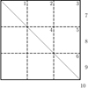 |
Fig. A.1. Generic form of the block-normalised covariance matrices SN and correlation matrices C. |
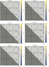 |
Fig. A.2. Block-normalised covariance matrices SN for the highest-fsv light curve regression models obtained for KIC003240411, KIC003459297, KIC003756031, KIC003839930, KIC003865742, and KIC004930889. The strategies that correspond to these highest-fsv light curve regression models are listed in the ‘Strategy’ columns in Tables 2 and 3. The normalisation values for each block are displayed at the locations specified in Fig. A.1. We note that the (one-cell-wide) blocks of (co)variances with the y intercept β0 are displayed at the bottom and right hand side of each panel. The change in darkness between the upper and lower triangular part of each matrix is aesthetic. |
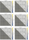 |
Fig. A.3. Same as Fig. A.2, but for KIC004936089, KIC004939281, KIC005084439, KIC0050309849, KIC005941844, and KIC006352430. |
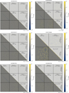 |
Fig. A.4. Same as Fig. A.2, but for KIC006462033, KIC006780397, KIC007630417, KIC007760680, KIC008057661, and KIC008087269. |
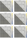 |
Fig. A.5. Same as Fig. A.2, but for KIC008255796, KIC008324482, KIC008381949, KIC008459899, KIC008714886, and KIC008766405. |
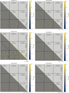 |
Fig. A.6. Same as Fig. A.2, but for KIC009020774, KIC009227988, KIC009715425, KIC009964614, KIC010220209, and KIC010285114. |
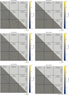 |
Fig. A.7. Same as Fig. A.2, but for KIC010526294, KIC010536147, KIC010658302, KIC01115422, KIC011360704, and KIC011454304. |
 |
Fig. A.9. Correlation matrices C for the highest-fsv light curve regression models obtained for KIC011971405 and KIC012258330. The strategies that correspond to these light curve regression models are listed in the ‘Strategy’ columns in Tables 2 and 3. Equation (A.4) delivers the explicit expressions used to compute the correlations within each block, which are displayed at the locations specified in Sect. A.4. The change in darkness between the upper and lower triangular part of each matrix is aesthetic. |
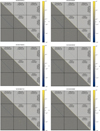 |
Fig. A.10. Same as Fig. A.9, but for KIC003240411, KIC003459297, KIC003756031, KIC003839930, KIC003865742, and KIC004930889. |
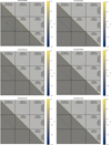 |
Fig. A.11. Same as Fig. A.9, but for KIC004936089, KIC004939281, KIC005084439, KIC005309849, KIC005941844, and KIC006352430. |
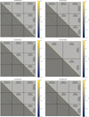 |
Fig. A.12. Same as Fig. A.9, but for KIC006462033, KIC006780397, KIC007630417, KIC007760680, KIC008057661, and KIC008087269. |
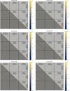 |
Fig. A.13. Same as Fig. A.9, but for KIC008255796, KIC008324482, KIC008381949, KIC008459899, KIC008714886, and KIC008766405. |
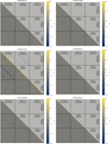 |
Fig. A.14. Same as Fig. A.9, but for KIC009020774, KIC009227988, KIC009715425, KIC009964614, KIC010220209, and KIC010285114. |
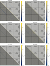 |
Fig. A.15. Same as Fig. A.9, but for KIC010526294, KIC010536147, KIC010658302, KIC011152422, KIC011360704, and KIC011454304. |
Appendix B: Light curve regression model selection and candidate resonance identification
In this appendix, we discuss the light curve regression model selection process and the number of identified candidate resonances for each individual star in our sample, noting the correspondence among the fsv values and the residual summary statistics shown in Fig. B.1. We show which pre-whitening strategies have the largest fsv values in Tables 2 and 3, for the high and low fsv stars, respectively. In those tables we also include the rotation rates obtained from averaging over eight theories of core-boundary and envelope mixing, derived by Pedersen et al. (2021), as well as an indication of the smallest unresolved signal in the residual LS periodogram, and the amplitude of the largest-amplitude signal that is resolved in the LS periodogram of the original light curve. Finally, we also provide an indication of which stars are binaries, and which stars exhibit outburst-like features in their light curves.
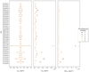 |
Fig. B.1. Comparison of the residual summary statistics for the different pre-whitening strategies applied to the stars in the sample. From left to right: Bayesian estimator for the residual bias |


Table B.1 provides the iterative pre-whitening step numbers at which the stop criteria are triggered for the five pre-whitening strategies applied to each of the 38 stars in our sample. In the following subsections we provide information on the light curve regression model selection and candidate resonance identification characteristics for the stars in each pseudo-class. We include an assessment of the priority for non-linear asteroseismic follow-up that is focused on FP solutions of the AEs, which is influenced by the number of robust candidate resonances that involve the 𝒩i largest-amplitude signals that are indicated in Table B.2.
Increasing the number of largest-amplitude signals that may be involved in a (second-order) detected candidate resonance, 𝒩i, in general changes the number of identified robust candidate resonances compared to the number of identified robust two-signal candidate resonances. Because we define robust candidate resonances in general to be unique matches in frequency to within 1 Rayleigh limit at the 1σ level, similar to the definition of a two-signal candidate resonance given in Eq. (9), there are two (competing) effects that can be noted when increasing 𝒩i. Firstly, the number of extracted signals with which a candidate resonance can be formed increases, hence increasing the total number of identified candidate resonances. Secondly, the chance that candidate resonances have non-unique identifiers increases. As one expects the probability for a resonance to occur increases with oscillation amplitude, the first effect is also influenced by oscillation amplitudes. Both effects counterbalance each other in a manner that is star-dependent, as can be noted from the number of identified robust candidate resonances in Table B.2. We note that we only consider second-order candidate resonances in this work, which for some stars provides an upper bound for 𝒩i: any further increase in 𝒩i above this bound would result in the detection of higher-order candidate resonances.
The conservative approach used in Sect. 4.1 to identify two-signal candidate resonances provides one with a first account of the typical number of robust candidate identified within the light curve regression models of SPB stars. This number of identified candidate resonances stays fairly consistent if 𝒩i is varied. The number of two-signal candidate resonances therefore is a good indicator for selecting prime targets for non-linear asteroseismic follow-up, as it indicates which stars display the most robust candidate resonances.
B.1. High-fsv stars
B.1.1. Generic characteristics
In correspondence with the high fsv values attained by the light curve regression models for the high-fsv stars, the variance left in the residuals is low for almost all of these stars. The high mode densities within the LS periodograms do however leave some signals unresolved by the LD78 resolution, so that a non-noise-level variance is expected. KIC010526294 is an extreme example of the effect of such a high mode density: although the attained fsv values tend to ∼ 97% for all five pre-whitening strategies, we note a large variance left in its residuals, as shown in Fig. B.1. For most high-fsv stars the unresolved signals are not of such high amplitude. No significant residual light curve bias is observed for any of the high-fsv stars.
We find many high-fsv stars to exhibit robust two-signal candidate resonances, as shown in Table 4. Imposing the additional S/N ≥ 5 criterion lowers the amount of robust two-signal candidate resonances detected, reducing the number of stars that exhibit such candidate resonances by five. Even with this reduction in number, many of them display robust candidate resonances, and are therefore prime targets for non-linear asteroseismic follow-up, as indicated in Table B.2.
B.1.2. Individual discussion
KIC003459297 was identified as an SPB star by Pápics et al. (2017), and frequency analysis was performed by Pápics et al. (2017), Christophe et al. (2018) and Szewczuk et al. (2021). Multiple mode-dense regions can be noted in its LS periodogram. Pápics et al. (2017) note that many of the frequencies not in the mode dense region around 1 d−1 can be explained by combination frequencies. However, only one robust candidate resonance is detected (see Table B.2), for which S/N ≥ 5, making this star a low-priority target for follow-up.
KIC003839930 was first identified as an SPB star by Balona et al. (2011) and McNamara et al. (2012), and its variability was analysed by Szewczuk et al. (2021). Its variability is dominated by signals that have frequencies < 2 d−1. We find one robust two-signal candidate resonance, which becomes non-robust for larger 𝒩i. Other robust candidate resonances are identified, which involve smaller-amplitude signals and mostly have S/N values ≥ 5, hence, this star has a medium priority for follow-up.
Iterative pre-whitening steps at which the stop criteria trigger for each of the five pre-whitening strategies applied to all 38 SPB stars in our sample.
Number of robust candidate resonances that involve the 𝒩i largest-amplitude signals for each star in our sample, and the priorities for non-linear asteroseismic follow-up.
KIC003865742 was first identified as an SPB star by McNamara et al. (2012). Its LS periodogram displays high-mode-density groups and very-large-amplitude signals below 0.5 d−1, with large-amplitude signals being found below 1.5 d−1. Many robust candidate resonances can be identified, although this decreases with increasing 𝒩i, and many have S/N values < 5. Moreover, higher-order candidate resonances can also be identified, giving this star a medium priority for follow-up.
KIC004930889 was first identified as an SPB star and SB2 binary by Pápics et al. (2017), who also analysed the system’s variability. The mode density in its LS periodogram is grouped, and these groups contain the largest-amplitude signals. We find many robust candidate resonances, of which none pass the additional S/N ≥ 5 criterion, and also identify higher-order candidate resonances. Hence, this star has a low priority for follow-up.
KIC004936089 was first classified as an SPB star by McNamara et al. (2012), and its variability was analysed in Szewczuk et al. (2021). Its LS periodogram contains high-mode-density groups, yet, we identify few robust candidate resonances, which all have S/N ≥ 5. We do not find higher-order candidate resonances. Hence, this star has a high priority for follow-up.
KIC005084439 was first classified as an SPB star by McNamara et al. (2012). We note high-mode-density groups in its LS periodogram and we detect several robust candidate resonances, which all have S/N ≥ 5. Because we also identify higher-order candidate resonances, this star has a medium priority for follow-up.
KIC005309849 was found to be a misidentified B star by Zhang et al. (2018). Its LS periodogram is mode dense, and contains a large-amplitude low-frequency signal. Although we identify several robust candidate resonances of which many have S/N ≥ 5, we also detect higher-order candidate resonances, hence, a medium priority for follow-up is assigned.
KIC005941844 was discussed as an example high-fsv star in the main text. It is a high-priority target for non-linear asteroseismic follow-up, because it exhibits many robust candidate resonances, of which several have S/N ≥ 5. We also detect no higher-order candidate resonances.
KIC006352430 was first identified as an SPB star and SB2 binary by Pápics et al. (2013). It has a very rich LS periodogram, in which low-amplitude signals can be noted at very low frequencies (below 0.5 d−1) that can be attributed to the orbital period harmonics (Pápics et al. 2013). Alternatively, these frequencies can be identified as difference frequencies (Pápics et al. 2017), because of the high mode density within the LS periodogram. Our regression models include most of these frequencies (strategies 1 and 4), or all of them (strategies 2, 3, 5). We find many robust candidate resonances, of which half have S/N ≥ 5, but also detect higher-order candidate resonances, making this star a medium priority target only.
KIC006780397 was first identified as an SPB star by McNamara et al. (2012). Most of the variability within its LS periodogram can be found at frequencies < 1.5 d−1, forming a mode-dense region that includes the largest-amplitude pulsations for this star. Several of the detected two-signal candidate resonances are robust, but only a few have S/N ≥ 5, and we also detect higher-order candidate resonances. This star thus has a medium priority for follow-up.
KIC007760680 was first identified as an SPB star by Pápics et al. (2015). Its LS periodogram displays high-mode-density groups. Pápics et al. (2015) detected a period spacing pattern tilted by rotation and affected by internal mixing. This pattern was analysed in more detail by Moravveji et al. (2016) to set asteroseismic constraints on core overshooting and mixing. We detect several robust candidate resonances, of which many have S/N ≥ 5, but also find higher-order candidate resonances, giving this star a medium priority for follow-up.
KIC008324482 was identified to be a misclassified B-star by Zhang et al. (2018). Its LS periodogram displays a high-mode-density group. We find several robust candidate resonances, of which most have S/N ≥ 5, and detect no higher-order candidate resonances, giving this star a high priority for follow-up.
KIC008714886 was first identified as an SPB star by Balona et al. (2011), and its variability was analysed by Szewczuk et al. (2021). Pedersen et al. (2021) note that it is the only star within their sample of 26 SPB stars that exhibits retrograde modes. We note high-mode-density regions in its LS periodogram. We also detect many robust candidate resonances, and no higher-order resonances. KIC008714886 therefore is a high-priority target for follow-up.
KIC008766405 was first identified as an SPB star by McNamara et al. (2012). We note several high-mode-density groups in its LS periodogram. Furthermore, we identify a large number of robust candidate resonances of which many have S/N ≥ 5, and no higher-order resonances. KIC008766405 therefore is a high-priority target for follow-up.
KIC009020774 was first identified as an SPB star by Pápics et al. (2017). We note mode dense regions in its LS periodogram. Few robust candidate resonances are identified of which few have S/N ≥ 5, and higher-order candidate resonances are noted. It is therefore a low-priority target for follow-up.
KIC009227988 was first identified as an SPB star by McNamara et al. (2012), and its variability was analysed by Szewczuk et al. (2021). The variability of this star dominantly resides below 1 d−1. Few robust candidate resonances are identified, and none have S/N ≥ 5. Because we also note higher-order candidate resonances, this star is a low-priority target for follow-up.
KIC010220209 was first identified as an SPB star by McNamara et al. (2012). Several mode-dense groups are noted in its LS periodogram. Interestingly, strategy 5 fails to deliver a model in which candidate resonances are detected, whereas the other strategies have no such issues. We note no robust candidate resonances. It is therefore a low-priority target for follow-up.
KIC010526294 was first identified as an SPB star by Debosscher et al. (2011) and McNamara et al. (2012). It is, together with KIC008459899 and KIC008255796, the slowest rotator in our sample, which is differentially rotating (Triana et al. 2015). Its variability was analysed by Pápics et al. (2015) and Szewczuk et al. (2021). It was the subject of detailed asteroseismic modelling focused on inferring internal mixing in Moravveji et al. (2015). The LS periodogram displays the largest-amplitude signal noted in any of the SPB stars in our sample. It also displays regions of high mode density around the largest-amplitude modes in which several relatively large-amplitude unresolved signals (with respect to the LD78 resolution) can be found among the rotationally split dipole triplets. This is the only star in the sample with rotational multiplets. Many robust candidate resonances are identified, and most have S/N ≥ 5, whereas no higher-order resonances are noted. Hence, this star has a high priority for follow-up.
KIC010658302 was first identified as an SPB star by Balona et al. (2011) and McNamara et al. (2012). We note distinct high-mode-density groups in its LS periodogram. We find few robust candidate resonances of which most have S/N ≥ 5, but also identify no higher-order resonances. This star therefore has a medium priority for follow-up.
B.2. High-mode-density stars
B.2.1. Generic characteristics
The variances retained in the residual light curves of high-mode-density stars are not significantly larger than those of high-fsv stars. No high-mode-density stars exhibit any residual light curve bias, as shown in Fig. B.1.
The average rotation rate of a high-mode-density star is larger than that of a high-fsv star. Whether this implies that one or more physical factors are at play that cause this difference, remains to be verified. It could be that some of these stars are for example quiescent/inactive Be stars, as was claimed by Rivinius et al. (2016) for KIC008057661.
B.2.2. Individual discussion
KIC003240411 was determined to be ‘the hottest known SPB star with a asymptotic g-mode spacing’ by Szewczuk & Daszyńska-Daszkiewicz (2018) while studying its variability. Its residual LS periodogram shows that a single unresolved large-amplitude signal that is unresolved with respect to the LD78 resolution, is causing the low fsv values associated with the generated light curve regression models. The appearance of the large-amplitude unresolved signal, close to the dominant frequency, is furthermore a marker indicating that this frequency’s amplitude is modulated, as was noted by Szewczuk & Daszyńska-Daszkiewicz (2018). Only one robust candidate resonance is identified (see Table B.2), which has S/N ≥ 5. KIC003240411 is therefore a low-priority target for follow-up.
KIC003756031 was classified as a (hybrid) SPB star by Balona et al. (2011) and McNamara et al. (2012). We identify several robust candidate resonances among the many signals in the high-mode-density LS periodogram, of which several have S/N ≥ 5. However, we also identify higher-order candidate resonances, giving this target a medium priority for follow-up.
KIC006462033 was identified as a misclassified B star by Zhang et al. (2018). The residual LS periodogram is mode-dense, with small-amplitude signals crowding the frequency range spanning ∼0 to ∼5 days. No robust candidate resonances are noted, and higher-order resonances are detected, giving this star a low priority for follow-up.
KIC007630417 was originally classified as an SPB stars by McNamara et al. (2012), whereas Szewczuk et al. (2021) classified it as a hybrid pulsator while analysing its variability. The (low-amplitude) LS periodogram is rich in signals, and we detect many robust candidate resonances, several of which have S/N ≥ 5. Because we also detect no higher-order candidate resonances, this star has a high priority for follow-up.
KIC008057661 was first classified as a (hybrid) SPB star by Balona et al. (2011), whereas Rivinius et al. (2016) classified it as an inactive Be star. We note a mode-dense region at lower frequencies in its LS periodogram. We find several robust candidate resonances and several have S/N ≥ 5, but also detect higher-order resonances. Hence, we attribute a medium priority for follow-up.
KIC008087269 was first classified as an SPB star by McNamara et al. (2012). Distinct high-mode-density groups are noted in its LS periodogram. We identify a few robust candidate resonances, of which many have S/N ≥ 5. We also detect higher-order resonances, however, so that a medium priority for follow-up is assigned.
The LS periodogram of KIC008255796, the high-mode-density star example discussed in the main text, has mode-dense groups. We identify several robust candidate resonances for KIC008255796, for which none have S/N ≥ 5, which can be explained by the high mode density in its LS periodogram. Because we also identify higher-order resonances, it gets a low priority for follow-up.
KIC008381949 was first classified as a (hybrid) SPB pulsator by Balona et al. (2011), and its variability was analysed by Szewczuk et al. (2021). It has a rich LS periodogram, in which mode-dense regions and large-amplitude signals can be noted. The amplitude modulation observed in Szewczuk et al. (2021) is therefore expected. We find several robust candidate resonances of which several have S/N ≥ 5 (see Table B.2), and detect no higher-order resonances. Because of the observed amplitude modulation, this star only gets a medium priority for follow-up.
KIC008459899 was first classified as an SPB star by Balona et al. (2011), and, as noted in Sect. 3.2, it is suspected to be an SB2 system (Lehmann et al. 2011). Its LS periodogram is mode-dense in the ∼0 to ∼2 d−1 region. Only a few robust candidate resonances are detected of which approximately half have S/N ≥ 5, and higher-order resonances are identified. Hence, this star has a low priority for follow-up.
KIC009964614 was first classified as a (hybrid) SPB star by Balona et al. (2011), and its variability was analysed by Szewczuk et al. (2021). Its LS periodogram has a mode-dense region below 1 d−1. We find some robust candidate resonances, and a few have S/N ≥ 5, but also identify higher-order resonances at higher values of 𝒩i. KIC009964614 therefore has a low priority for follow-up.
KIC010536147 was first classified as an SPB pulsator by Balona et al. (2011). Its LS periodogram is crowded (mode-dense) within the region ∼0 to ∼5 d−1. We find several robust candidate resonances for this star, yet, not many have S/N ≥ 5, and we also identify higher-order resonances. Hence, it only has a medium priority for follow-up.
KIC011454304 was first classified as an SPB star by Balona et al. (2011) and McNamara et al. (2012). Its LS periodogram is mode-dense especially in the frequency region covering ∼0.25 to ∼1.25 d−1. We identify only one robust candidate resonance (for which S/N ≥ 5), and note no higher-order resonances. This star thus has a medium priority for follow-up.
KIC012258330 was first classified as a (hybrid) SPB star by Lehmann et al. (2011). Its LS periodogram is mode-dense, especially in those regions that also contain large-amplitude signals. Several robust candidate resonances are identified, of which approximately half have S/N ≥ 5, and no higher-order resonances are noted. Hence, this target has a high priority for follow-up.
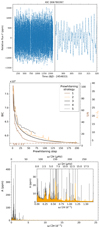 |
Fig. B.10. Same as Fig. 3, but for KIC006780397. |
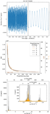 |
Fig. B.11. Same as Fig. 3, but for KIC007760680. |
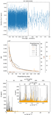 |
Fig. B.12. Same as Fig. 3, but for KIC008324482. |
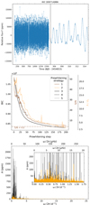 |
Fig. B.13. Same as Fig. 3, but for KIC008714886. |
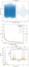 |
Fig. B.14. Same as Fig. 3, but for KIC008766405. |
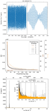 |
Fig. B.15. Same as Fig. 3, but for KIC009020774. |
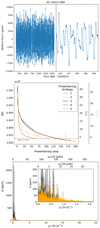 |
Fig. B.16. Same as Fig. 3, but for KIC009227988. |
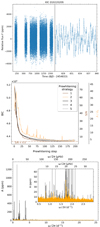 |
Fig. B.17. Same as Fig. 3, but for KIC010220209. |
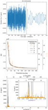 |
Fig. B.18. Same as Fig. 3, but for KIC010526294. |
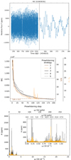 |
Fig. B.19. Same as Fig. 3, but for KIC010658302. |
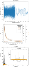 |
Fig. B.20. Same as Fig. 3, but for KIC003240411. |
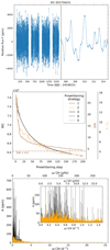 |
Fig. B.21. Same as Fig. 3, but for KIC003756031. |
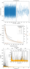 |
Fig. B.22. Same as Fig. 3, but for KIC006462033. |
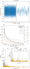 |
Fig. B.23. Same as Fig. 3, but for KIC007630417. |
 |
Fig. B.24. Same as Fig. 3, but for KIC008057661. |
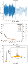 |
Fig. B.25. Same as Fig. 3, but for KIC008087269. |
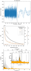 |
Fig. B.26. Same as Fig. 3, but for KIC008381949. |
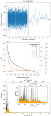 |
Fig. B.27. Same as Fig. 3, but for KIC008459899. |
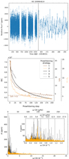 |
Fig. B.28. Same as Fig. 3, but for KIC009964614. |
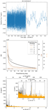 |
Fig. B.29. Same as Fig. 3, but for KIC010536147. |
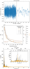 |
Fig. B.30. Same as Fig. 3, but for KIC011454304. |
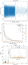 |
Fig. B.31. Same as Fig. 3, but for KIC012258330. |
B.3. Outbursting stars
B.3.1. Generic characteristics
The variances retained in the residual light curves of 3 outbursting stars (KIC004939281, KIC010285114 and KIC011152422) are not significantly larger than those of high-fsv stars, in contrast to the 3 stars that display (very) large variances in their residual light curves, KIC009715425, KIC011360704 and KIC011971405. No outbursting stars exhibit any residual light curve bias, as shown in Fig. B.1.
The large rotation rates observed for the outbursting low-fsv stars are reminiscent of the rotation rates for classical Be stars, fitting the average classical Be star rotation rate (> 80% critical) noted in Rivinius et al. (2013). All outbursting stars have a low priority for non-linear asteroseismic follow-up.
B.3.2. Individual discussion
KIC004939281 was classified as an SPB star by McNamara et al. (2012), whose variability was analysed by Szewczuk et al. (2021). The outburst-like feature displayed in its light curve is long, spanning several months. High-mode-density groups are noted in its LS periodogram. We find no robust candidate resonances and identify higher-order resonances at larger 𝒩i.
KIC009715425 was first classified as an SPB star by McNamara et al. (2012), whose variability was analysed in Szewczuk et al. (2021). Its LS periodogram contains several high-mode-density groups. We find few to no robust candidate resonances (which have S/N ≥ 5), and identify higher-order resonances.
KIC010285114 was first classified as a (hybrid) SPB pulsator by Balona et al. (2011) and McNamara et al. (2012). Its LS periodogram contains several high-mode-density groups. Few to no robust candidate resonances are identified, which have S/N ≥ 5.
KIC011152422 was first classified as an SPB star by McNamara et al. (2012). Some structure can be identified in the LS periodogram, which may be attributed to the short time base of the light curve. We identify some robust candidate resonances, of which only half have S/N ≥ 5, but also identify larger-order resonances.
KIC011360704 was first classified as a (hybrid) SPB star by McNamara et al. (2012), whose variability was analysed by Szewczuk et al. (2021). Distinct high-mode-density groups are noted in its LS periodogram. Many robust candidate resonances are identified, but only a few have S/N ≥ 5. Moreover, we also identify higher-order resonances, which together with its outburst-like features in the light curve, ensure the low priority for follow-up.
We identify few robust candidate resonances for KIC011971405, the example outbursting star discussed in the main text. Several of these have S/N ≥ 5. Similar to KIC010285114, no higher-order resonances are identified.
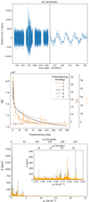 |
Fig. B.32. Same as Fig. 3, but for KIC004939281. |
 |
Fig. B.33. Same as Fig. 3, but for KIC009715425. |
 |
Fig. B.34. Same as Fig. 3, but for KIC010285114. |
 |
Fig. B.35. Same as Fig. 3, but for KIC011152422. |
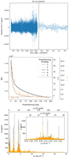 |
Fig. B.36. Same as Fig. 3, but for KIC011360704. |
All Tables
Rotation rates (Ωrot/Ωcrit, Pedersen et al. 2021), highest-fsv pre-whitening strategies, and symbolic largest-amplitude ratio (Aunres/res) for the 19 high-fsv stars, if applicable.
Number of two-signal candidate resonances for each of the five pre-whitening strategies applied to all stars in our sample, and the number of two-signal candidate resonances defined as ‘robust’.
Iterative pre-whitening steps at which the stop criteria trigger for each of the five pre-whitening strategies applied to all 38 SPB stars in our sample.
Number of robust candidate resonances that involve the 𝒩i largest-amplitude signals for each star in our sample, and the priorities for non-linear asteroseismic follow-up.
All Figures
|
Fig. 1. Comparison of the scaled fraction of variance fsv values of the resulting light curve regression models obtained for the different pre-whitening strategies applied to the stars in the sample, with colouring as a function of fsv. Each cell contains the fsv value as computed using Eq. (3), as well as the total number of frequencies extracted using this approach, ne. The number ne and the fsv value are computed after the frequency filtering step has removed any unresolved frequencies with respect to the LD78 criterion and any signals that have insignificant amplitudes (at 95% confidence), as discussed in Sect. 2.2. |
| In the text | |
|
Fig. 2. Total percentage of explained scaled variance fsv averaged over all 38 stars in the sample (‘all stars’) for each of the five pre-whitening strategies. This averaged percentage is also displayed for each of the three pseudo-classes introduced in Sect. 3. |
| In the text | |
|
Fig. 3. Light curve, pre-whitening and pulsation characteristics for the high-fsv star KIC005941844. Top: full light curve (left) and a small part of the light curve that indicates its multi-periodic constant-frequency nature (right). Middle: comparison of the different stop criteria used for the five pre-whitening strategies throughout the iterative pre-whitening procedure, applied to the light curve. The BIC values are relevant for strategies 3, 4, and 5, whereas the S/N value and the estimated amplitude A expressed in estimated standard deviations |
| In the text | |
|
Fig. 4. Distribution of the amplitudes and frequencies of (independent) signals not identified as combination frequencies for all 38 SPB stars in our sample, for each of the pre-whitening strategies defined in Table 1. The colour indicates if these signals are involved in a candidate resonance (red) or not (blue), and its gradient indicates the number of detected frequencies: Colours are brighter if more signals are detected within a specific amplitude-frequency bin. The red and blue distributions are plotted independently, so overlap between these distributions is the cause for the appearance of darker, maroon-like coloured bins belonging to the red distribution. The maximal frequency displayed in each panel is 8 d−1, which is the highest frequency of any of the detected (robust two-signal) candidate resonances (see Sect. 4 and, especially, Fig. 10). We display independent signals with an amplitude > 10 ppm because very few independent signals have amplitudes smaller than this limit. |
| In the text | |
|
Fig. 5. Box-and-whisker plot of the rotation rates of 26 SPB stars obtained from averaging over eight theories of core-boundary and envelope mixing by Pedersen et al. (2021). These are grouped into the two classes defined in this work: low and high fsv, as indicated schematically on the x axis. Whiskers are extended past the quartiles by maximally 1.5 times the interquartile range. Outliers are indicated with a rhombus mark. Individual rotation rates and estimated standard deviations are indicated in grey. The horizontal offset for these rotation rates is imposed for reasons of visibility, without any additional meaning. |
| In the text | |
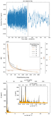 |
Fig. 6. Same as Fig. 3, but for high-mode-density star KIC008255796. |
| In the text | |
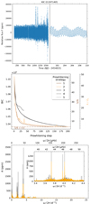 |
Fig. 7. Same as Fig. 3, but for outbursting star KIC011971405. |
| In the text | |
|
Fig. 8. Covariance matrix of the best regression model of the light curve of KIC005914844 (obtained from pre-whitening strategy 3) in the block-normalised form described in Appendix A.4 and Fig. A.1. The colour map shows the normalised (co)variance values (SN)ij, norm, and the change in darkness between the upper and lower triangular part of the matrix is only for visualisation purposes. |
| In the text | |
|
Fig. 9. Box-and-whisker plots of the number of identified two-signal candidate resonances or the number of identified robust two-signal candidate resonances (defined by Eq. (9)), grouped by the pseudo-classes defined in this work: low and high fsv. Left panel: box-and-whisker plot of the number of identified two-signal candidate resonances. The colour depicts the pre-whitening strategy employed to generate the light curve models. Right panel: box-and-whisker plot of the number of identified robust two-signal candidate resonances. Whiskers and outliers for both panels are indicated in a similar way to how they are indicated in Fig. 5. |
| In the text | |
|
Fig. 10. Highest-fsv strategy characteristic properties of the identified robust candidate resonances, which involve the two largest-amplitude signals, as a function of each other, with 1σ uncertainties indicated: amplitude A, frequency ω/2π, frequency de-tuning δν (see Eq. (4)), relative phase Φ (see Eq. (5)), and relative amplitude Ar (see Eq. (6)). Colours indicate the different pseudo-classes to which the stars that exhibit the candidate resonances belong. The transparent symbols indicate robust candidate resonances having 4 < S/N < 5, whereas the full symbols indicate robust candidate resonances for which S/N ≥ 5. Grey lines indicate the zero point for the frequency de-tuning, and the faint grey horizontal lines in the last row of panels indicate the relative phases that satisfy Eq. (5). |
| In the text | |
|
Fig. A.1. Generic form of the block-normalised covariance matrices SN and correlation matrices C. |
| In the text | |
|
Fig. A.2. Block-normalised covariance matrices SN for the highest-fsv light curve regression models obtained for KIC003240411, KIC003459297, KIC003756031, KIC003839930, KIC003865742, and KIC004930889. The strategies that correspond to these highest-fsv light curve regression models are listed in the ‘Strategy’ columns in Tables 2 and 3. The normalisation values for each block are displayed at the locations specified in Fig. A.1. We note that the (one-cell-wide) blocks of (co)variances with the y intercept β0 are displayed at the bottom and right hand side of each panel. The change in darkness between the upper and lower triangular part of each matrix is aesthetic. |
| In the text | |
|
Fig. A.3. Same as Fig. A.2, but for KIC004936089, KIC004939281, KIC005084439, KIC0050309849, KIC005941844, and KIC006352430. |
| In the text | |
|
Fig. A.4. Same as Fig. A.2, but for KIC006462033, KIC006780397, KIC007630417, KIC007760680, KIC008057661, and KIC008087269. |
| In the text | |
|
Fig. A.5. Same as Fig. A.2, but for KIC008255796, KIC008324482, KIC008381949, KIC008459899, KIC008714886, and KIC008766405. |
| In the text | |
|
Fig. A.6. Same as Fig. A.2, but for KIC009020774, KIC009227988, KIC009715425, KIC009964614, KIC010220209, and KIC010285114. |
| In the text | |
|
Fig. A.7. Same as Fig. A.2, but for KIC010526294, KIC010536147, KIC010658302, KIC01115422, KIC011360704, and KIC011454304. |
| In the text | |
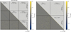 |
Fig. A.8. Same as Fig. A.2, but for KIC011971405 and KIC012258330. |
| In the text | |
|
Fig. A.9. Correlation matrices C for the highest-fsv light curve regression models obtained for KIC011971405 and KIC012258330. The strategies that correspond to these light curve regression models are listed in the ‘Strategy’ columns in Tables 2 and 3. Equation (A.4) delivers the explicit expressions used to compute the correlations within each block, which are displayed at the locations specified in Sect. A.4. The change in darkness between the upper and lower triangular part of each matrix is aesthetic. |
| In the text | |
|
Fig. A.10. Same as Fig. A.9, but for KIC003240411, KIC003459297, KIC003756031, KIC003839930, KIC003865742, and KIC004930889. |
| In the text | |
|
Fig. A.11. Same as Fig. A.9, but for KIC004936089, KIC004939281, KIC005084439, KIC005309849, KIC005941844, and KIC006352430. |
| In the text | |
|
Fig. A.12. Same as Fig. A.9, but for KIC006462033, KIC006780397, KIC007630417, KIC007760680, KIC008057661, and KIC008087269. |
| In the text | |
|
Fig. A.13. Same as Fig. A.9, but for KIC008255796, KIC008324482, KIC008381949, KIC008459899, KIC008714886, and KIC008766405. |
| In the text | |
|
Fig. A.14. Same as Fig. A.9, but for KIC009020774, KIC009227988, KIC009715425, KIC009964614, KIC010220209, and KIC010285114. |
| In the text | |
|
Fig. A.15. Same as Fig. A.9, but for KIC010526294, KIC010536147, KIC010658302, KIC011152422, KIC011360704, and KIC011454304. |
| In the text | |
|
Fig. B.1. Comparison of the residual summary statistics for the different pre-whitening strategies applied to the stars in the sample. From left to right: Bayesian estimator for the residual bias |
| In the text | |
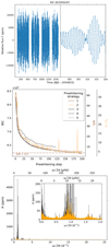 |
Fig. B.2. Same as Fig. 3, but for KIC003459297. |
| In the text | |
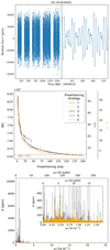 |
Fig. B.3. Same as Fig. 3, but for KIC003839930. |
| In the text | |
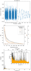 |
Fig. B.4. Same as Fig. 3, but for KIC003865742. |
| In the text | |
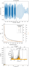 |
Fig. B.5. Same as Fig. 3, but for KIC004930889. |
| In the text | |
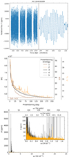 |
Fig. B.6. Same as Fig. 3, but for KIC004936089. |
| In the text | |
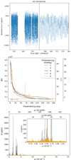 |
Fig. B.7. Same as Fig. 3, but for KIC005084439. |
| In the text | |
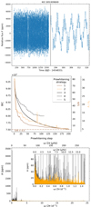 |
Fig. B.8. Same as Fig. 3, but for KIC005309849. |
| In the text | |
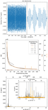 |
Fig. B.9. Same as Fig. 3, but for KIC006352430. |
| In the text | |
|
Fig. B.10. Same as Fig. 3, but for KIC006780397. |
| In the text | |
|
Fig. B.11. Same as Fig. 3, but for KIC007760680. |
| In the text | |
|
Fig. B.12. Same as Fig. 3, but for KIC008324482. |
| In the text | |
|
Fig. B.13. Same as Fig. 3, but for KIC008714886. |
| In the text | |
|
Fig. B.14. Same as Fig. 3, but for KIC008766405. |
| In the text | |
|
Fig. B.15. Same as Fig. 3, but for KIC009020774. |
| In the text | |
|
Fig. B.16. Same as Fig. 3, but for KIC009227988. |
| In the text | |
|
Fig. B.17. Same as Fig. 3, but for KIC010220209. |
| In the text | |
|
Fig. B.18. Same as Fig. 3, but for KIC010526294. |
| In the text | |
|
Fig. B.19. Same as Fig. 3, but for KIC010658302. |
| In the text | |
|
Fig. B.20. Same as Fig. 3, but for KIC003240411. |
| In the text | |
|
Fig. B.21. Same as Fig. 3, but for KIC003756031. |
| In the text | |
|
Fig. B.22. Same as Fig. 3, but for KIC006462033. |
| In the text | |
|
Fig. B.23. Same as Fig. 3, but for KIC007630417. |
| In the text | |
|
Fig. B.24. Same as Fig. 3, but for KIC008057661. |
| In the text | |
|
Fig. B.25. Same as Fig. 3, but for KIC008087269. |
| In the text | |
|
Fig. B.26. Same as Fig. 3, but for KIC008381949. |
| In the text | |
|
Fig. B.27. Same as Fig. 3, but for KIC008459899. |
| In the text | |
|
Fig. B.28. Same as Fig. 3, but for KIC009964614. |
| In the text | |
|
Fig. B.29. Same as Fig. 3, but for KIC010536147. |
| In the text | |
|
Fig. B.30. Same as Fig. 3, but for KIC011454304. |
| In the text | |
|
Fig. B.31. Same as Fig. 3, but for KIC012258330. |
| In the text | |
|
Fig. B.32. Same as Fig. 3, but for KIC004939281. |
| In the text | |
|
Fig. B.33. Same as Fig. 3, but for KIC009715425. |
| In the text | |
|
Fig. B.34. Same as Fig. 3, but for KIC010285114. |
| In the text | |
|
Fig. B.35. Same as Fig. 3, but for KIC011152422. |
| In the text | |
|
Fig. B.36. Same as Fig. 3, but for KIC011360704. |
| In the text | |
Current usage metrics show cumulative count of Article Views (full-text article views including HTML views, PDF and ePub downloads, according to the available data) and Abstracts Views on Vision4Press platform.
Data correspond to usage on the plateform after 2015. The current usage metrics is available 48-96 hours after online publication and is updated daily on week days.
Initial download of the metrics may take a while.