| Issue |
A&A
Volume 658, February 2022
|
|
|---|---|---|
| Article Number | A37 | |
| Number of page(s) | 8 | |
| Section | The Sun and the Heliosphere | |
| DOI | https://doi.org/10.1051/0004-6361/202141505 | |
| Published online | 28 January 2022 | |
Toward a fast and consistent approach to modeling solar magnetic fields in multiple layers
1
Key Laboratory of Solar Activity, National Astronomical Observatories, Chinese Academy of Sciences, Beijing, PR China
e-mail: xszhu@bao.ac.cn
2
Max-Planck-Institut für Sonnensystemforschung, Justus-von-Liebig-Weg 3, 37077 Göttingen, Germany
Received:
9
June
2021
Accepted:
19
September
2021
Aims. We aim to develop a fast and consistent extrapolation method for modeling multiple layers of the solar atmosphere.
Methods. The new approach combines the magnetohydrostatic (MHS) extrapolation, which models the solar low atmosphere in a flat box, together with the nonlinear force-free field (NLFFF) extrapolation, which models the solar corona with a chromospheric vector magnetogram deduced from the MHS extrapolation. We tested our code with a snapshot of a radiative magnetohydrodynamic simulation of a solar flare and we conducted quantitative comparisons based on several metrics.
Results. Following a number of test runs, we found an optimized configuration for the combination of two extrapolations with a 5.8-Mm-high box for the MHS extrapolation and a magnetogram at a height of 1 Mm for the NLFFF extrapolation. The new approach under this configuration has the capability to reconstruct the magnetic fields in multi-layers accurately and efficiently. Based on figures of merit that are used to assess the performance of different extrapolations (NLFFF extrapolation, MHS extrapolation, and the combined one), we find the combined extrapolation reaches the same level of accuracy as the MHS extrapolation and they are both better than the NLFFF extrapolation. The combined extrapolation is moderately efficient for application to magnetograms with high resolution.
Key words: Sun: magnetic fields / Sun: photosphere / Sun: chromosphere / Sun: corona
© ESO 2022
1. Introduction
Over half a century, numerous extrapolations have been developed to compute magnetic fields from the photosphere to the corona (see reviews by Régnier 2013; Wiegelmann & Sakurai 2021). As one of the most frequently used extrapolation methods in modeling coronal magnetic fields of an active region, a nonlinear force-free field (NLFFF) extrapolation assumes a vanishing Lorentz force in the solar corona in which the plasma β is very low. Then the coronal magnetic fields can be described by


Taking the divergence of Eq. (1) and using Eq. (2), we get

showing α is constant along each magnetic field line but can have different values on different field lines. In the lower atmosphere, however, magnetic field is not necessarily force-free due to non-negligible gas pressure gradient and gravity. The non-force-freeness of the magnetic field in the lower atmosphere was confirmed by a number of studies (Metcalf et al. 1995; Moon et al. 2002; Tiwari 2012; Liu et al. 2013; Liu & Hao 2015), which showed that most photospheric magnetograms of active regions fail to fulfill the Aly’s criteria (Molodenskii 1969; Molodensky 1974; Aly 1984, 1989) for a force-free field. The inconsistency between the force-free assumption and the non-force-free magnetogram has prevented NLFFF extrapolations from acquiring good results (Metcalf et al. 2008; De Rosa et al. 2009).
To overcome this issue of inconsistency, we may perform the NLFFF extrapolation by using a chromospheric magnetogram. It was found that the magnetic field becomes force-free roughly 400 km above the photosphere (Metcalf et al. 1995). However, the chromosphere is thicker than the photosphere and chromospheric spectrum lines are formed across a wide range of heights (Bjørgen et al. 2019), which makes it difficult to tell at which height a magnetogram is located. Moreover, interpreting spectropolarimetric measurements made using chromospheric spectrum lines is still a challenge (Harvey 2012). Another way to deal with the inconsistency is to preprocess the photospheric magnetogram before it is applied. Wiegelmann et al. (2006) first proposed an algorithm to modify magnetogram within the error margins of measurement to minimize the net magnetic force and torque in the data. After that, several other preprocessing methods were developed (Fuhrmann et al. 2007; Tadesse et al. 2009; Yamamoto & Kusano 2012; Jiang & Feng 2014). The preprocessed magnetogram is much more suitable for a NLFFF extrapolation than the unpreprocessed one. The third way, which seems more straightforward, is to design the magnetohydrostatic (MHS) extrapolation to solve the following MHS equations:

where B, p, ρ, and g are the magnetic field, plasma pressure, plasma density, and gravitational acceleration, respectively. The magnetic fields and plasma interact consistently in the MHS extrapolation, which allows the photospheric magnetogram to not fulfill Aly’s criteria. The MHS extrapolations have been developed based on magnetohydrodynamic relaxation method (Zhu et al. 2013, 2016; Miyoshi et al. 2020), Grad & Rubbin (1958) method (Gilchrist & Wheatland 2013; Gilchrist et al. 2016), and optimization method (Wiegelmann & Neukirch 2006; Wiegelmann et al. 2007; Zhu & Wiegelmann 2018, 2019). Applications of the MHS extrapolation mainly focus on activities in the low atmosphere (Zhao et al. 2017; Tian et al. 2018; Chen et al. 2019; Song et al. 2020; Zhu et al. 2016, 2017, 2020a; Jafarzadeh et al. 2021).
It is worth noting that a new class of the NLFFF extrapolations by using multiple observations has been recently introduced (Malanushenko et al. 2012; Aschwanden 2013; Chifu et al. 2015; Dalmasse et al. 2019). Besides the photospheric magnetogram, these extrapolations take advantage of either EUV images (AIA, Lemen et al. 2012) or coronal polarimetric observations (CoMP, Tomczyk et al. 2008). As we obtain more and more data, such as polarimetric observation with various wavelengths by DKIST (Tritschler et al. 2016) and radio observation with various frequencies by MUSER (Yan et al. 2009, 2021), that are sensitive to magnetic fields, it is a promising way to optimize the extrapolation process with multiple observations.
In this work, we try to address two issues: the first one to validate the effectiveness of the MHS extrapolation applied to the solar corona and the second to improve the efficiency of the MHS extrapolation, which has been found rather time-consuming. The reference solution is a snapshot of a radiative MHD (RMHD) simulation of a solar flare, which has been used to test the MHS extrapolation in the lower solar atmosphere (Zhu & Wiegelmann 2019). The remainder of the paper is organized as follows. The reference solution is described in Sect. 2. The application of the MHS extrapolation to the corona is tested in Sect. 3. An incorporation of the two extrapolations are tested in Sect. 4. Our conclusions are presented in Sect. 5.
2. Active region in an RMHD simulation
Cheung et al. (2019) carried out an RMHD simulation of a solar flare along with a coronal mass ejection. The RMHD code includes 3D radiative transfer in the convection zone and photosphere, along with optically thin radiation and field-aligned heat conduction in the corona, which mimics a realistic environment on the Sun. The eruption of the simulation was triggered by imposing an emergence of a twisted flux rope into a pair of initially potential sunspots.
As the reference model, we chose a snapshot that was eight minutes after flare peak. The reference model was previously used to test the MHS extrapolation in the lower atmosphere (Zhu & Wiegelmann 2019). The original data spans ±49.2(±24.6 Mm) in x (y) axis and spans from 7.5 Mm beneath the photosphere to 41.6 Mm above in z axis. The grid resolution is 192 km in the horizontal directions and 64 km in the vertical. The photospheric magnetogram (Fig. 1a) is located at the average geometrical height, corresponding to optical depth unity. In Figs. 1b and c, we show magnetic field lines from different perspectives. We see that the top of the flux rope is roughly 10 Mm in the low solar corona, which is much higher than chromospheric structures, which typically have a height of 2 Mm.
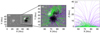 |
Fig. 1. Reference model for testing the extrapolation. (a): Photospheric magnetogram. (b): Sample magnetic field lines in the white box outlined in panel a. Purple (green) lines are open (closed) magnetic field lines. (c) Same field lines seen from south. |
Although the system was still dynamic at the moment of the reference snapshot, we found out that the time-varying term is at least one order of magnitude smaller than the other terms in the moment equation (see Fig. 1a of Zhu & Wiegelmann 2019). Figure 2 shows influence of magnetic pressure (Pb = B2/2), plasma pressure (p), and inertial term (Pv = ρv2) at different layers. We see the plasma pressure is the most important term in the very low atmosphere (below 250 km), while the magnetic term dominates the higher layers. Recall that the MHS model does not consider the inertial force. Hence, the snapshot of the RMHD simulation serves an adequate reference model to test our code.
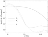 |
Fig. 2. Horizontal averages of the reference model. Pb (solid line), Pv (dotted line), and p (dashed line) are horizontally averaged magnetic pressure, inertial term, and plasma pressure, respectively. |
We also checked the magnetogram to see to what degree it satisfies with criteria for either a force-free or a MHS state. The Aly critera (Molodenskii 1969; Molodensky 1974; Aly 1984, 1989), which consist of six integrals on the magnetogram, are necessary conditions for the magnetic field to be force-free. They are given by
where S1 is the bottom boundary. Equations (6)–(8) represent the null net Lorentz force at each of three directions, while Eqs. (9)–(11) represent the null net Lorentz force torque at each of three directions. The necessary conditions for the magnetic field to be in a MHS state are weaker because of the existence of plasma (Zhu et al. 2020b), which only consist of the Eqs. (6), (7), and (11). Moreover, based on the Eqs. (6), (7), and (11), Zhu et al. (2020b) developed a preprocessing procedure to remove the net transverse forces and vertical torque on magnetogram, while the net vertical force and transverse torques remain. The preprocessed magnetogram is consistent with the MHS assumption and, hence, it is supposed to be more appropriate for a MHS extrapolation. Figure 3 shows changes of scaled net Lorentz force and torque along height. We can see Fx/F0, Fy/F0, Tz/T0 are very close to zero in all layers while Fz/F0, Tx/T0, Ty/T0 are around 0.1 in the photosphere, which means the Eqs. (6), (7), and (11) are satisfied well, while the vertical force and transverse torques are somewhat large. Therefore, the magnetogram may be used in the MHS extrapolation directly but should be preprocessed before being used in the NLFFF extrapolation. It is also worth noting that Fz/F0, Tx/T0, Ty/T0 decrease quickly and almost vanish above 400 km.
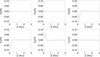 |
Fig. 3. Scaled net Lorentz force and torque with |
3. MHS extrapolation testing in the solar corona
3.1. Methodology and numerical setting
To solve the MHS Eqs. (4) and (5), we construct the functional
with
![$$ \begin{aligned}&{\boldsymbol{\Omega }_{a}} = \left[(\nabla \times \boldsymbol{B})\times \boldsymbol{B}-\nabla p - \rho {\hat{\boldsymbol{z}}}\right]/(B^2+p),\end{aligned} $$](/articles/aa/full_html/2022/02/aa41505-21/aa41505-21-eq15.gif)
![$$ \begin{aligned}&{\boldsymbol{\Omega }_{b}} = [(\nabla \cdot \boldsymbol{B})\boldsymbol{B}]/(B^2+p), \end{aligned} $$](/articles/aa/full_html/2022/02/aa41505-21/aa41505-21-eq16.gif)
where ωa and ωb are the weighting functions which are set to unity over the whole region in this study, ν is the Lagrangian multiplier. Bobs are the observed magnetic fields in the photosphere. W is a diagonal matrix to incorporate measurement error of the magnetic field. We set the vertical component wlos to unity, while the transverse component  . It is obvious that Eqs. (4) and (5) are fulfilled when L = 0. By using the gradient descent method the functional L is minimized. We note that to simplify the formulae (13), coefficients
  and g disappear due to appropriate normalization of physical quantities. For example, for a study that includes photosphere, the following normalization constants are convenient: ρ0 = 2.7 × 10⁻¹ g cm−3 (density), T0 = 6 × 10³ K (temperature), g = 2.7 × 104 cm s−2 (gravitational acceleration),
  cm (length),
  dyn cm−2 (plasma pressure), and
  G (magnetic field), where ℛ is the ideal gas constant.
The extrapolation follows the same dimensions of the reference model with 512 × 256 × 652 grid points in the (x, y, z) directions and with a grid spacing of 192 km horizontally and 64 km vertically. In a previous study (Zhu & Wiegelmann 2019), we used a flat box with 98 × 49 × 8 Mm3 to test the code in the chromosphere. The computational box is extended to the corona in this study.
As the initial condition we compute a NLFFF by an optimization method (Wiegelmann 2004) with the preprocessed magnetogram (Wiegelmann et al. 2006). During the NLFFF step, the preprocessed magnetogram is injected slowly (Wiegelmann & Inhester 2010). By slow injection, the potential field at the boundary adjusted continuously according to the gradient descent method over the total iterations of the calculation (usually a few thousand steps). Then we move to the next step of taking into account the effects of plasma forces. In this step, however, the original magnetogram is injected slowly. The side and upper boundaries of the magnetic field and the plasma are fixed to their initial values. The iteration stops when  for 500 consecutive steps. For more details of the implementation of the algorithm, we refer to Zhu & Wiegelmann (2018, 2019).
3.2. Results
To assess the quantify of the extrapolation results, we used six metrics, as introduced by Schrijver et al. (2006) and Barnes et al. (2006). These figures quantify the agreement between vector fields, namely, b of the reconstruction and B of the reference model.
Vector correlation
Cauchy-Schwarz inequality
Normalized vector error
Mean vector error
where N is the number of grid points in the computation box.
Field line divergence (FLD) metric: Tracing field lines from a random point on the bottom boundary in both reference model and extrapolation. If both field lines end again on the bottom boundary, a score, pi, can be given to this point with the distance between the two endpoints divided by the length of the field line in the reference model. Then a single score can be assigned by the fraction of the area in which pis are less than 10%. An alternative score can be given by the fraction of flux.
We chose a small volume for comparison to focus on the compact region and minimize boundary effects as well. The Cvec, CCS, EN, and EM were applied to the white box of Fig. 1 with a height of 30 Mm. The FLD metric traces field lines from each photospheric point in the green box of Fig. 1a. We note that those traced lines may pass out of the green box. Table 1 shows results of runs with various ν. We find, within a reasonable range of ν, the MHS extrapolation performs stably. A large ν forces the bottom boundary to agree with observation by compromising on balance of magnetic and non-magnetic forces. If ν is too small, deviation between the bottom boundary and observation can be large thus the result will be decoupled from the magnetogram. The choice ν = 0.001 seems the optimal and is used in the following modeling.
Metrics for the MHS extrapolations with various ν.
In the detailed analysis of the test that ensues, with the optimal ν, we divided the domain into two height ranges, [0, 10] Mm and [10, 30] Mm. The comparison in the lower region is focused mainly on the flux rope, while the higher region comparison is focused mainly on the ambient potential field. The quantitative evaluations are given in Table 2. The MHS extrapolation scores better than the NLFFF extrapolation in almost all metrics in both height ranges. In the higher region, the two extrapolations perform similarly to each other. The biggest difference among all metrics is less than 3.8%. The magnetic fields in this region consist of long and open loops which are nearly current-free. They can be well reconstructed even by a potential field extrapolation (De Rosa et al. 2009).
Metrics for the two extrapolations applied to the vector magnetogram of the flare simulation.
The comparison in the lower region, however, shows somewhat larger difference between the two extrapolations. Metrics EN and EM show that the MHS solution is 6% better than the NLFFF solution. These two metrics are sensitive to both angle and norm differences of the magnetic field while Cvec and CCS are sensitive to angle difference only. Among all metrics we used, the FLDs are the most rigorous two. The MHS extrapolation scores 0.72/0.76 in the two metrics, which are dramatic improvements (> 40%) over the NLFFF’s scores of 0.51/0.55. Although the angel and norm differences of the magnetic field are small in general, differences in the magnetic connectivity could be significant because of the accumulation of deviation when lines are traced. In Fig. 4, we compare the reference model with various extrapolation models. The MHS extrapolation shows better agreement with the reference model than the NLFFF extrapolation both in field lines pattern and connectivity. The magnetic field connectivity is crucial to explain eruptions and determine regions where reconnection is possible (Joshi et al. 2019).
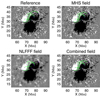 |
Fig. 4. Magnetic field configurations of different models. The same start points marked with rhombus are selected for all panels. End points of the referenced field lines are marked with circles. Magnetogram of the NLFFF extrapolation is smoother than other panels due to preprocession. |
The MHS extrapolation costs 14 h on the run with Intel Xeon Gold 6150 CPU (18 cores), while the NLFFF extrapolation only costs 0.2 h. The low convergence speed of the MHS extrapolation brings difficulties in modeling temporal evolution of the magnetic fields with high-spatial-resolution magnetogram (e.g., DIKST, GST).
4. Incorporation of two extrapolations
The above test showed that the MHS extrapolation works well in both the chromosphere and corona. However, the extremely low efficiency will obstruct its application to high spatial resolution magnetograms with a large field of view. Considering that the non-force-free region is thin, with a height less than 2 Mm (Metcalf et al. 1995; Zhu et al. 2016, 2020a), it is a straightforward step to apply the MHS extrapolation only to the low part (including the non-force-free region plus small part of force-free region), while the force-free corona is modeled by the NLFFF extrapolation. As the MHS solution includes a consistent transition from non-force-free to force-free regions, we can cut it transversely to get a vector magnetogram at a force-free height. The vector magnetogram will be used as the bottom boundary for the NLFFF extrapolation. At this point, we are faced with two issues, namely: the height at which we should cut the MHS solution to get a suitable magnetogram and how thin the computational box should be set for the MHS extrapolation to achieve a suitable magnetogram.
4.1. Determining the bottom boundary for the NLFFF extrapolation
The magnetic fields throughout the entire region do not necessarily become force-free at the same height. We can, of course, get a transverse slice of the MHS solution well within the corona to ensure its force-free quality at any location for the following NLFFF extrapolation. However, high-altitude slices require a relatively high computational box of the MHS extrapolation, which results in a limited improvement of computational efficiency. Therefore, the slice should be force-free and, at the same time, as low as possible. Figure 5 shows how magnetograms at different heights influence extrapolation results. Poor performance can be seen when magnetograms near the bottom plane are used. As using higher-altitude magnetograms, the results improve quickly and finally converge. We consider h = 1 Mm (marked with rhombuses) as an optimal height of the force-free vector magnetogram, above which the extrapolation shows no significant improvement.
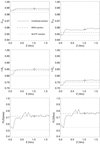 |
Fig. 5. Figures of merit for comparison (below 30 Mm) of the reference model and the combined extrapolation with magnetograms at various heights as boundary. The dashed and dotted lines show results of the NLFFF extrapolation and the MHS extrapolation, respectively. The optimal height 1 Mm is marked with the rhombus. |
4.2. Determining the height of computational box for the MHS extrapolation
In the above subsection, we find through tests that a magnetogram at h = 1 Mm is an optimal choice to link two extrapolations. Therefore the final question to be answered is how thin the computational box of the MHS extrapolation can be set. The MHS extrapolation in the above subsection is done in a 98 × 49 × 42 Mm box, which is computationally expensive. In this subsection, we aim to find out the optimal height of the box for the MHS extrapolation. The box should be, at one hand low enough to reduce computation amount and, on another hand, high enough to suppress upper boundary affection. Figure 6 shows how heights of the MHS extrapolation box influence extrapolation results. Upper boundary affection is obvious for a flat box with a height smaller than 4 Mm roughly. We consider h = 5.8 Mm (marked with rhombuses) as an optimal height of the MHS extrapolation box. A higher box does not lead to any significant improvement in the result. It is worth noting that the FLD indexes in both Figs. 5 and 6 show larger oscillations than those of other indexes, which might be due to nonlinearity of the tracing process. However, the trend of change is obvious.
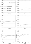 |
Fig. 6. Figures of merit for comparison (below 30 Mm) of the reference model and the combined extrapolation with various heights of the MHS extrapolation box. The magnetogram at 1 Mm is used as boundary input to the NLFFF extrapolation. The optimal height 5.8 Mm is marked with rhombus. |
4.3. Algorithm of the combined extrapolation
The current version of our code works as follows: (1) Perform a MHS extrapolation (Zhu & Wiegelmann 2018, 2019) by using an observed magnetogram within a 5.8-Mm-high box; (2) Cut the MHS solution at h = 1 Mm to get a magnetogram; (3) Perform a NLFFF extrapolation (Wiegelmann 2004) by using the synthetic magnetogram we note that the synthetic chromospheric magnetogram is force-free and smooth enough to not need preprocessing; and (4) Combine the MHS solution below 1 Mm and the NLFFF solultion together to create a new solution.
The above approach to the extrapolation costs two hours in runtime for the case in this study, which is seven times faster than the original MHS extrapolation. The improvement in efficiency is consistent with the choose of 5.8-Mm-high box, which is roughly one seventh of the height of the original MHS extrapolation box (42 Mm).
5. Conclusion
In this study, we have validated the MHS extrapolation with a snapshot of an RMHD simulation. Results have shown that the MHS extrapolation is more accurate than the NLFFF extrapolation to model the multiple layers on the Sun. However, it requires a much longer computational time. A new approach which combines the MHS extrapolation and the NLFFF extrapolation reaches the accuracy of the former one and, at the same time, inherits the efficiency of the later one. It is worth noting that in the above test, we used only one snapshot (post-flare) as the reference model. To show the robustness of our method, we also selected a pre-flare snapshot (30 min before flare) to further test the method. We find, based on the quantitative comparison showed in Table 3 for the additional test, that both the MHS extrapolation and the combined approach work well. Conclusions from the post-flare case test still hold in the pre-flare case.
Metrics for extrapolations with pre-flare reference model.
For active region 11768, observed by SUNRISE/IMaX (Martínez Pillet et al. 2011), with spatial resolution of 100 km and pixel spacing of 40 km, the 2000 × 2000 × 1280 box spans a volume of 80 × 80 × 51 Mm3 and roughly contains the main magnetic structure. With above grid points setting, the NLFFF extrapolation costs 10 h to complete, the MHS extrapolation costs 550 h, and the combined extrapolation costs 70 h. The combined extrapolation is moderately efficient for application to magnetograms with high resolution.
Acknowledgments
This work is supported by the mobility program (M-0068) of the Sino-German Science Center. TW acknowledges DLR-grant 50 OC 2101.
References
- Aly, J. J. 1984, ApJ, 283, 349 [NASA ADS] [CrossRef] [Google Scholar]
- Aly, J. J. 1989, Sol. Phys., 120, 19 [NASA ADS] [CrossRef] [Google Scholar]
- Aschwanden, M. J. 2013, ApJ, 763, 115 [NASA ADS] [CrossRef] [Google Scholar]
- Barnes, G., Leka, K. D., & Wheatland, M. S. 2006, ApJ, 641, 1188 [NASA ADS] [CrossRef] [Google Scholar]
- Bjørgen, J. P., Leenaarts, J., Rempel, M., et al. 2019, A&A, 631, A33 [Google Scholar]
- Chen, Y., Tian, H., Zhu, X., et al. 2019, Sci. China E: Technol. Sci., 62, 1555 [CrossRef] [Google Scholar]
- Cheung, M. C. M., Rempel, M., Chintzoglou, G., et al. 2019, Nat. Astron., 3, 160 [NASA ADS] [CrossRef] [Google Scholar]
- Chifu, I., Inhester, B., & Wiegelmann, T. 2015, A&A, 577, A123 [NASA ADS] [CrossRef] [EDP Sciences] [Google Scholar]
- Dalmasse, K., Savcheva, A., Gibson, S. E., et al. 2019, ApJ, 877, 111 [NASA ADS] [CrossRef] [Google Scholar]
- De Rosa, M. L., Schrijver, C. J., Barnes, G., et al. 2009, ApJ, 696, 1780 [NASA ADS] [CrossRef] [Google Scholar]
- Fuhrmann, M., Seehafer, N., & Valori, G. 2007, A&A, 476, 349 [NASA ADS] [CrossRef] [EDP Sciences] [Google Scholar]
- Gilchrist, S. A., & Wheatland, M. S. 2013, Sol. Phys., 282, 283 [NASA ADS] [CrossRef] [Google Scholar]
- Gilchrist, S. A., Braun, D. C., & Barnes, G. 2016, Sol. Phys., 291, 3583 [NASA ADS] [CrossRef] [Google Scholar]
- Grad, H., & Rubbin, H. 1958, in Theoretical and Experimental Aspects of Controlled Nuclear Fusion, eds. J. H. Martens, L. Ourom, W. M. Barss, et al., 31, 190 [Google Scholar]
- Harvey, J. W. 2012, Sol. Phys., 280, 69 [NASA ADS] [CrossRef] [Google Scholar]
- Jafarzadeh, S., Wedemeyer, S., Fleck, B., et al. 2021, Philos. Trans. R. Soc. London Ser. A, 379, 20200174 [NASA ADS] [Google Scholar]
- Jiang, C., & Feng, X. 2014, Sol. Phys., 289, 63 [NASA ADS] [CrossRef] [Google Scholar]
- Joshi, N. C., Zhu, X., Schmieder, B., et al. 2019, ApJ, 871, 165 [NASA ADS] [CrossRef] [Google Scholar]
- Lemen, J. R., Title, A. M., Akin, D. J., et al. 2012, Sol. Phys., 275, 17 [Google Scholar]
- Liu, S., & Hao, J. 2015, Adv. Space Res., 55, 1563 [NASA ADS] [CrossRef] [Google Scholar]
- Liu, S., Su, J. T., Zhang, H. Q., et al. 2013, PASA, 30, e005 [CrossRef] [Google Scholar]
- Malanushenko, A., Schrijver, C. J., DeRosa, M. L., Wheatland, M. S., & Gilchrist, S. A. 2012, ApJ, 756, 153 [NASA ADS] [CrossRef] [Google Scholar]
- Martínez Pillet, V., Del Toro Iniesta, J. C., Álvarez-Herrero, A., et al. 2011, Sol. Phys., 268, 57 [Google Scholar]
- Metcalf, T. R., Jiao, L., McClymont, A. N., Canfield, R. C., & Uitenbroek, H. 1995, ApJ, 439, 474 [NASA ADS] [CrossRef] [Google Scholar]
- Metcalf, T. R., De Rosa, M. L., Schrijver, C. J., et al. 2008, Sol. Phys., 247, 269 [Google Scholar]
- Miyoshi, T., Kusano, K., & Inoue, S. 2020, ApJS, 247, 6 [NASA ADS] [CrossRef] [Google Scholar]
- Molodenskii, M. M. 1969, Sov. Astron., 12, 585 [NASA ADS] [Google Scholar]
- Molodensky, M. M. 1974, Sol. Phys., 39, 393 [CrossRef] [Google Scholar]
- Moon, Y. J., Choe, G. S., Yun, H. S., Park, Y. D., & Mickey, D. L. 2002, ApJ, 568, 422 [NASA ADS] [CrossRef] [Google Scholar]
- Régnier, S. 2013, Sol. Phys., 288, 481 [CrossRef] [Google Scholar]
- Schrijver, C. J., De Rosa, M. L., Metcalf, T. R., et al. 2006, Sol. Phys., 235, 161 [NASA ADS] [CrossRef] [Google Scholar]
- Song, Y., Tian, H., Zhu, X., et al. 2020, ApJ, 893, L13 [NASA ADS] [CrossRef] [Google Scholar]
- Tadesse, T., Wiegelmann, T., & Inhester, B. 2009, A&A, 508, 421 [NASA ADS] [CrossRef] [EDP Sciences] [Google Scholar]
- Tian, H., Zhu, X., Peter, H., et al. 2018, ApJ, 854, 174 [NASA ADS] [CrossRef] [Google Scholar]
- Tiwari, S. K. 2012, ApJ, 744, 65 [NASA ADS] [CrossRef] [Google Scholar]
- Tomczyk, S., Card, G. L., Darnell, T., et al. 2008, Sol. Phys., 247, 411 [Google Scholar]
- Tritschler, A., Rimmele, T. R., Berukoff, S., et al. 2016, Astron. Nachr., 337, 1064 [Google Scholar]
- Wiegelmann, T. 2004, Sol. Phys., 219, 87 [NASA ADS] [CrossRef] [Google Scholar]
- Wiegelmann, T., & Inhester, B. 2010, A&A, 516, A107 [NASA ADS] [CrossRef] [EDP Sciences] [Google Scholar]
- Wiegelmann, T., & Neukirch, T. 2006, A&A, 457, 1053 [NASA ADS] [CrossRef] [EDP Sciences] [Google Scholar]
- Wiegelmann, T., & Sakurai, T. 2021, Liv. Rev. Sol. Phys., 18, 1 [NASA ADS] [CrossRef] [Google Scholar]
- Wiegelmann, T., Inhester, B., & Sakurai, T. 2006, Sol. Phys., 233, 215 [Google Scholar]
- Wiegelmann, T., Neukirch, T., Ruan, P., & Inhester, B. 2007, A&A, 475, 701 [NASA ADS] [CrossRef] [EDP Sciences] [Google Scholar]
- Yamamoto, T. T., & Kusano, K. 2012, ApJ, 752, 126 [NASA ADS] [CrossRef] [Google Scholar]
- Yan, Y., Zhang, J., Wang, W., et al. 2009, Earth Moon Planets, 104, 97 [CrossRef] [Google Scholar]
- Yan, Y., Chen, Z., Wang, W., et al. 2021, Front. Astron. Space Sci., 8, 584043 [Google Scholar]
- Zhao, J., Schmieder, B., Li, H., et al. 2017, ApJ, 836, 52 [Google Scholar]
- Zhu, X., & Wiegelmann, T. 2018, ApJ, 866, 130 [NASA ADS] [CrossRef] [Google Scholar]
- Zhu, X., & Wiegelmann, T. 2019, A&A, 631, A162 [NASA ADS] [CrossRef] [EDP Sciences] [Google Scholar]
- Zhu, X. S., Wang, H. N., Du, Z. L., & Fan, Y. L. 2013, ApJ, 768, 119 [NASA ADS] [CrossRef] [Google Scholar]
- Zhu, X., Wang, H., Du, Z., & He, H. 2016, ApJ, 826, 51 [NASA ADS] [CrossRef] [Google Scholar]
- Zhu, X., Wang, H., Cheng, X., & Huang, C. 2017, ApJ, 844, L20 [NASA ADS] [CrossRef] [Google Scholar]
- Zhu, X., Wiegelmann, T., & Solanki, S. K. 2020a, A&A, 640, A103 [NASA ADS] [CrossRef] [EDP Sciences] [Google Scholar]
- Zhu, X., Wiegelmann, T., & Inhester, B. 2020b, A&A, 644, A57 [NASA ADS] [CrossRef] [EDP Sciences] [Google Scholar]
All Tables
Metrics for the two extrapolations applied to the vector magnetogram of the flare simulation.
All Figures
|
Fig. 1. Reference model for testing the extrapolation. (a): Photospheric magnetogram. (b): Sample magnetic field lines in the white box outlined in panel a. Purple (green) lines are open (closed) magnetic field lines. (c) Same field lines seen from south. |
| In the text | |
|
Fig. 2. Horizontal averages of the reference model. Pb (solid line), Pv (dotted line), and p (dashed line) are horizontally averaged magnetic pressure, inertial term, and plasma pressure, respectively. |
| In the text | |
|
Fig. 3. Scaled net Lorentz force and torque with |
| In the text | |
|
Fig. 4. Magnetic field configurations of different models. The same start points marked with rhombus are selected for all panels. End points of the referenced field lines are marked with circles. Magnetogram of the NLFFF extrapolation is smoother than other panels due to preprocession. |
| In the text | |
|
Fig. 5. Figures of merit for comparison (below 30 Mm) of the reference model and the combined extrapolation with magnetograms at various heights as boundary. The dashed and dotted lines show results of the NLFFF extrapolation and the MHS extrapolation, respectively. The optimal height 1 Mm is marked with the rhombus. |
| In the text | |
|
Fig. 6. Figures of merit for comparison (below 30 Mm) of the reference model and the combined extrapolation with various heights of the MHS extrapolation box. The magnetogram at 1 Mm is used as boundary input to the NLFFF extrapolation. The optimal height 5.8 Mm is marked with rhombus. |
| In the text | |
Current usage metrics show cumulative count of Article Views (full-text article views including HTML views, PDF and ePub downloads, according to the available data) and Abstracts Views on Vision4Press platform.
Data correspond to usage on the plateform after 2015. The current usage metrics is available 48-96 hours after online publication and is updated daily on week days.
Initial download of the metrics may take a while.