| Issue |
A&A
Volume 645, January 2021
|
|
|---|---|---|
| Article Number | A12 | |
| Number of page(s) | 28 | |
| Section | Extragalactic astronomy | |
| DOI | https://doi.org/10.1051/0004-6361/202039062 | |
| Published online | 21 December 2020 | |
The MURALES survey
III. Completing the MUSE observations of 37 3C low-z radio galaxies
1
INAF – Osservatorio Astrofisico di Torino, Via Osservatorio 20, 10025 Pino Torinese, Italy
e-mail: barbara.balmaverde@inaf.it
2
Dipartimento di Fisica e Astronomia, Università di Firenze, Via G. Sansone 1, 50019 Sesto Fiorentino, Firenze, Italy
3
INAF – Osservatorio Astrofisico di Arcetri, Largo Enrico Fermi 5, 50125 Firenze, Italy
4
Space Telescope Science Institute, 3700 San Martin Dr., Baltimore, MD 21210, USA
5
Johns Hopkins University, 3400 N. Charles Street, Baltimore, MD 21218, USA
6
INAF – Istituto di Radioastronomia, Via Gobetti 101, 40129 Bologna, Italy
7
INAF – Osservatorio di Astrofisica e Scienza dello Spazio di Bologna, Via Gobetti 93/3, 40129 Bologna, Italy
8
Department of Physics and Astronomy, University of Manitoba, Winnipeg, MB R3T 2N2, Canada
9
Leiden Observatory, Leiden University, PO Box 9513, 2300 RA Leiden, The Netherlands
10
Harvard-Smithsonian Center for Astrophysics, 60 Garden St., Cambridge, MA 02138, USA
11
University of Maryland Baltimore County, 1000 Hilltop Circle, Baltimore, MD 21250, USA
12
SETI Institute, 189 N. Bernado Ave, Mountain View CA, 94043, USA
13
Instituto de Astrofísica, Facultad de Física, Pontificia Universidad Católica de Chile, Casilla 306, Santiago 22, Chile
Received:
29
July
2020
Accepted:
30
September
2020
We present the final observations of a complete sample of 37 radio galaxies from the Third Cambridge Catalogue (3C) with redshift < 0.3 and declination < 20° obtained with the VLT/MUSE optical integral field spectrograph. These data were obtained as part of the MUse RAdio Loud Emission line Snapshot (MURALES) survey with the main goal of exploring the AGN feedback process in the most powerful radio sources. We present the data analysis and, for each source, the resulting emission line images and the 2D gas velocity field. Thanks to the unprecedented depth these observations reveal emission line regions (ELRs) extending several tens of kiloparsec in most objects. The gas velocity shows ordered rotation in 25 galaxies, but in several sources it is highly complex. We find that the 3C sources show a connection between radio morphology and emission line properties. In the ten FR I sources the line emission region is generally compact, only a few kpc in size; only in one case does it exceed the size of the host. Conversely, all but two of the FR II galaxies show large-scale structures of ionized gas. The median extent is 16 kpc with the maximum reaching a size of ∼80 kpc. There are no apparent differences in extent or strength between the ELR properties of the FR II sources of high and low gas excitation. We confirm that the previous optical identification of 3C 258 is incorrect: this radio source is likely associated with a quasi-stellar object at z ∼ 1.54.
Key words: galaxies: active / galaxies: jets / galaxies: ISM / galaxies: nuclei
© ESO 2020
1. Introduction
Radio galaxies (RGs), usually hosted by the brightest galaxies at the center of clusters or groups, are among the most energetic manifestations of supermassive black holes (SMBHs) in the Universe. The study of these objects has become particularly important due to their role in the feedback process, which is the exchange of matter and energy between AGN, their host galaxies, and clusters of galaxies. The evidence of AGN feedback mode is often witnessed in local RGs, showing the presence of cavities inflated by the radio emitting gas in the X-ray images (e.g., kinetic feedback; Bîrzan et al. 2004, 2020). However, we still lack a comprehensive view of the effects that the highly collimated jets and the nuclear emission have on the host and its immediate environment. In particular, it is still unclear how precisely the coupling between radio jets and ionized gas occurs, and whether the jets are able to accelerate the gas above the host escape velocity (McNamara & Nulsen 2007). We also lack clear observational evidence of the conditions under which jets enhance or quench star formation (positive or negative feedback, e.g., Fabian 2012). Furthermore, the mechanical luminosity released by the AGN is not well-constrained because it is estimated using indirect and model-dependent approaches (e.g., Blanton et al. 2011; Panagoulia et al. 2014). Finally, the radiative output from the AGN can produce fast outflows of ionized gas, which might also affect the properties of the ambient medium (e.g., Balmaverde et al. 2016; Wylezalek & Zakamska 2016; Carniani et al. 2016; Cresci & Maiolino 2018).
The AGN feedback action can be directly probed by studying the narrow-line region (NLR), a region of intense narrow emission lines that can usually be traced up to few kiloparsec from the nucleus. The size of the NLR correlates with the nuclear [O III] λ5007 Å (hereafter [O III]) luminosity as ![$ r \propto L_{\mathrm{[O~III]}}^{0.5} $](/articles/aa/full_html/2021/01/aa39062-20/aa39062-20-eq1.gif) (Bennert et al. 2002), suggesting that the gas is photoionized by the nucleus and that the ionization parameter scales with the distance. However, in some quasi-stellar objects (QSOs), the [O III] emission line has been detected up to 20 kpc or more (Wampler et al. 1975; Stockton 1976; Richstone & Oke 1977). This region, characterized by extended line emitting gas showing complex shape and kinematics, has been named the extended narrow-line region (ENLR). The properties of the nuclear and the extended gas are related, and there is a linear relation between the line and radio luminosities in extended RGs (Baum & Heckman 1989a,b; Rawlings et al. 1989; Rawlings & Saunders 1991; Buttiglione et al. 2010). Moreover, the luminosity and size of the ENLR also correlates with the nuclear Hα+[N II] or [O III] luminosity (Mulchaey et al. 1996). The expected trend between the extended emission line luminosity and total radio power, and between the size of the emission line region and redshift, have been found by other studies using HST data (e.g., Tremblay et al. 2009; Baldi et al. 2019; Privon et al. 2008). We can now re-explore these relations using the higher sensitivity of MUSE.
(Bennert et al. 2002), suggesting that the gas is photoionized by the nucleus and that the ionization parameter scales with the distance. However, in some quasi-stellar objects (QSOs), the [O III] emission line has been detected up to 20 kpc or more (Wampler et al. 1975; Stockton 1976; Richstone & Oke 1977). This region, characterized by extended line emitting gas showing complex shape and kinematics, has been named the extended narrow-line region (ENLR). The properties of the nuclear and the extended gas are related, and there is a linear relation between the line and radio luminosities in extended RGs (Baum & Heckman 1989a,b; Rawlings et al. 1989; Rawlings & Saunders 1991; Buttiglione et al. 2010). Moreover, the luminosity and size of the ENLR also correlates with the nuclear Hα+[N II] or [O III] luminosity (Mulchaey et al. 1996). The expected trend between the extended emission line luminosity and total radio power, and between the size of the emission line region and redshift, have been found by other studies using HST data (e.g., Tremblay et al. 2009; Baldi et al. 2019; Privon et al. 2008). We can now re-explore these relations using the higher sensitivity of MUSE.
In this context, the third Cambridge Catalogue of RGs (3C, Spinrad et al. 1985) represents the best testbed to explore these open problems. It covers a wide range of radio power; it contains all types of sources from the point of view of their optical spectrum and radio morphology, enabling us to perform statistically robust comparison among the various classes. In the last two decades a superb suite of ground- and space-based observations has been built for the 3C with all major observing facilities from HST to Chandra, Spitzer, Herschel, and JVLA.
In Balmaverde et al. (2018a) we presented a spectacular example of the capabilities of MUSE for this class of sources, discussing the observation of 3C 317, a radio galaxy located at the center of the Abell cluster A2052. We detected a complex network of emission lines filaments, enshrouding the northern cavity, extending out to ∼20 kpc. The emission line ratios in the filaments suggest ionization from slow shocks or from cosmic rays; we did not detect any star forming regions. Modeling the global kinematics, we derived a velocity expansion of ∼250 km s−1, a value we used to estimate the cavity age.
The MUse RAdio Loud Emission lines Snapshot (MURALES) project is a program aimed at observing the 3C radio sources with the Multi-Unit Spectroscopic Explorer (MUSE) at the Very Large Telescope (VLT) (Bacon et al. 2010). Our main goals are to study the feedback process in a sample of the most powerful radio sources, to constrain the coupling between the radio source and the warm gas, to probe the fueling process, and to estimate the net effect of the feedback on star formation. The MUSE data can be combined with the unique multi-band dataset available for these sources, produced with all major observing facilities at all accessible wavelengths, adding a key ingredient for our understanding of the radio-loud AGN phenomenon.
As a first step of MURALES, we started with the MUSE observations of the 3C sources with z < 0.3, accessible from the VLT (i.e., δ < 20°). We were recently awarded MUSE observing time to extend the sample to larger distances and radio power, observing a sample of 29 3C radio galaxies up to z = 0.8. In Balmaverde et al. (2019) we presented the results of the observations of the first 20 3C sources obtained in Period 99. Thanks to their unprecedented depth (the median 3σ surface brightness limit in the emission line maps at the [O III] wavelength is 6 × 10⁻¹⁸ erg s−1 cm−2 arcsec−2), these observations reveal extended emission line structures in most objects. We found that in three of the four Fanaroff & Riley (1974) Class I radio galaxies (FR Is), the line emission regions are compact, ∼1 kpc in size; in all but one of the FR IIs, we detect large-scale structures of ionized gas reaching sizes of up to ∼80 kpc.
The richness of the information stored in the MUSE datacubes enables us to investigate many different scientific questions that cannot be exhausted here. For example, we can obtain deep emission line images and compare them with the X-ray and radio structures; exploring the spatial link between the hot and warm ionized ISM phases, and with the radio outflows, could provide evidence of shocked regions of gas along the jets path and/or around the radio lobes. We can also derive spatially resolved emission line ratio maps to explore the gas physical conditions in order to detect star forming regions, in search of positive feedback. In addition, the profile of the emission lines can reveal evidence of nuclear outflows affecting large-scale environments.
We complete our survey by presenting the MUSE data of the remaining 17 sources, observed in Period 102. The paper is organized as follows. In Sect. 2 we present the sample observed, provide an observation log, and describe the data reduction. In Sect. 3 we describe the case of 3C 258. In Sect. 4 we present the properties of the extended emission line region and in Sect. 5 we show the resulting emission line images, line ratio maps, and 2D velocity fields. We also provide a description of the individual sources. The results are summarized in Sect. 6.
In two forthcoming papers we will study the properties of the extended emission line structures in order to explore their origin and their connection with the radio jets. We will also look for nuclear outflows of ionized gas.
We adopt the following set of cosmological parameters: Ho = 69.7 km s−1 Mpc−1 and Ωm = 0.286 (Bennett et al. 2014).
2. Observations and data reduction
We observed a sample of 37 RGs with MUSE as part of the MURALES survey. The sample is formed of all the 3C radio-sources limited to z < 0.3 and δ < 20°. The information on the first subset of 20 objects was presented by Balmaverde et al. (2019); in this paper we complete the analysis of the remaining 17 3C sources. The main properties of the galaxies are listed in Table 1. The full sample covers the redshift range 0.003 < z < 0.289, with 21 sources located at z < 0.1. Their radio power spans more than four orders of magnitude, from ∼1031 to ∼1035 erg s−1 at 178 MHz. Most of them (26) are FR II. RGs are also separated into spectroscopic classes depending on the relative strength of the diagnostic optical emission lines (Hine & Longair 1979; Laing et al. 1994); we used the classification obtained by Buttiglione et al. (2010, 2011). All classes (low excitation galaxies, LEGs; high excitation galaxies, HEGs; and broad-line objects, BLOs) are represented with an almost equal share of LEGs (including six FR II/LEGs) and HEGs or BLOs. We compare the redshift and radio power distribution of our sample with that of the entire population of 114 3C RGs at z < 0.3 presented by Buttiglione et al. (2009). The mean redshift and radio power are z = 0.09 and log L178 = 33.69 erg s−1, respectively, not dissimilar from the values measured for the entire 3C subsample with z < 0.3 (z = 0.13 and log L178 = 33.61 erg s−1). The Kolmogorov–Smirnov test confirms that the two distributions of z and L178 are not statistically distinguishable. Our subsample can then be considered representative of the population of powerful, low redshift RGs.
Main properties of the 3C subsample observed with MUSE, and the observations log.
The observations presented here were obtained as part of the program ID 0102.B-0048(A). Two exposures of 10 min each were obtained with the VLT/MUSE spectrograph between November 5, 2018, and March 11, 2019 with the nominal wavelength range (4800–9300 Å). The median seeing of the observations is  , the same value of the first set of observations. We split the total on-source exposure time into two sub-exposures, applying a 5″ dithering pattern and a 90 degree rotation between on-object exposures to reject cosmic rays. We used the ESO MUSE pipeline (version 1.6.2; Weilbacher et al. 2020) to obtain fully reduced and calibrated data cubes. Summarizing, the pipeline corrects for the bias, the flat, and the vignetting; removes cosmic rays; calibrates each exposure in wavelength and in flux; and subtracts the sky background. For the flux calibration of the image, the pipeline uses a pre-processed spectrophotometric standard star observation. A known issue of the MUSE calibration procedure is that the astrometry in some cases is not precise. We used the position of bright sources in the MUSE field observed by Pan-STARRs to correct for any astrometric offset.
We followed the same strategy for the data analysis described in Balmaverde et al. (2018b), producing flux, velocity, and velocity dispersion maps for all the emission lines in the spectrum. However, in this paper, we focus on the brightest and most spatially extended emission line (Hα, [N II], or [O III]).
3. The case of 3C 258
The radio source 3C 258 was identified as a galaxy at redshift z = 0.165 (Wyndham 1966). This value was challenged by Dey (1994) who noted the likely presence of a background quasar, but, due to poor seeing of the observations, no firm claims can be made. The NICMOS/HST images by Floyd et al. (2008) are consistent with the higher redshift as they show a very compact host galaxy, much fainter than expected for an object at z = 0.165. The superposition of the radio image from Neff et al. (1995) on the MUSE continuum image indicates that what had been identified as the optical counter part is actually offset by  at PA = −20° (see Fig. 1). A point-like object is seen at the location of the radio source, also in the optical HST (de Koff et al. 1996) and Chandra images (Massaro et al. 2012). The MUSE spectrum of this object shows a single emission line, with a broad profile, at λ = 7116 Å. The most likely identification of this line is Mg II at λ2798 Å, confirming the Dey (1994) result and suggesting a tentative association with a type I AGN at z ∼ 1.54: at this redshift the MUSE spectrum covers the rest frame range ∼1900 − 3600 Å, a spectral region devoid of strong emission lines. We will not consider this object further in our analysis.
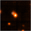 |
Fig. 1. Radio contours (white) of 3C 258 from Neff et al. (1995) superimposed on the optical continuum image (field of view 25″ × 25″) derived from the MUSE data. The radio source is offset by |

4. Luminosities and sizes of the ELR
In Table 1 we list the measurements of sizes and luminosities of the ELR measured in the 37 sources of the sample. We consider separately the central (i.e., within a radius of 3 times the seeing of the observations) and the extended component. The size of the ELR is measured as the largest radius at which emission lines are detected above the 3σ level. ELRs are considered to be not resolved when they do not extend beyond a radius of 3 times the seeing: this occurs in five FR Is and in two FR IIs.
The top panel of Fig. 2 compares the luminosities of the nucleus and of the extended ELR: they are linked by a strong correlation with a slope consistent with unity and a median ratio of LNuc/LExt ∼ 2. We estimated the Pearson partial and semi-partial correlation coefficient, finding that the correlation is significant (> 95%); we obtained a null probability value of 0.037 (partial correlation probability) and 0.024 (semi-partial probability value) after removing the common dependence of luminosities on redshift. We verified that a similarly tight correlation is also present considering the nuclear and extended line fluxes. An apparently similar connection is found between the radio power and the extended line luminosity (see the second panel), reminiscent of the correlation between the extended and nuclear ELR luminosities just discussed and the well-known link between the line and radio luminosities in extended RGs (Baum & Heckman 1989a,b; Rawlings et al. 1989; Rawlings & Saunders 1991; Buttiglione et al. 2010). However, by applying the statistical tests just described, we found that this relation is mainly driven by the common dependence on redshift, and it is not significant. In the third panel of Fig. 2 we explore the dependence on redshift of the extended luminosity Hα+[N II]. The expected positive trend (because going to higher redshifts we select more powerful sources able to ionize much more gas) is indeed observed. The bottom panel shows a positive trend, albeit with a large spread, between the size and the luminosity of the ELRs. The distribution of the sources in this plane could be consistent with the behavior expected from photoionization of a central source (i.e.,  ), as already found in Seyfert galaxies and QSOs (e.g., Bennert et al. 2002; Husemann et al. 2014; Sun et al. 2018; Chen et al. 2019).
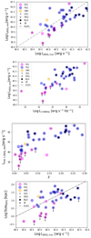 |
Fig. 2. From top to bottom, first and second panels: logarithm of the luminosities of the extended ELRs in the [N II] line vs. nuclear line luminosity and radio luminosities (all quantities in erg s−1). Sources are coded with symbols combining the optical spectroscopic classification and radio morphology. The dashed line is the bisectrix of the plane. Third panel: luminosity of the Hα+[N II] emission line vs. redshift. Fourth panel: logarithm of the size of the extended ELR (in kpc) vs. nuclear line luminosity. The dashed line shows the |

Overall, the ten FR Is are (with the exception of 3C 348, or Hercules A, a source with a hybrid FRI/FRII morphology) associated with the less luminous (and smaller) ELRs. When compared to the FR IIs, they show a large deficit in luminosity (a factor ≳10) and in size (a factor ≳3) of the extended ELR at given nuclear luminosity.
Conversely, there is no clear separation in terms of size and luminosity of the extended ELRs between the various spectroscopic classes among the FR IIs. Those of the BLO subclass have the more luminous central ELR, but the size and luminosity of their EELRs are similar to those seen in the FR IIs/HEGs and LEGs. This is likely due to the effects of the circumnuclear selective obscuration on the NLR (Baldi et al. 2013; Baum et al. 2010). The comparison of the HEG/BLO1 and LEG classes is limited by the small number of the LEG/FR IIs (six objects) and we cannot perform a robust statistical analysis. Nonetheless, HEG-BLO and LEG/FR II cover the same ranges in power and size of the extended ELRs. In particular, we find two LEG/FR IIs (3C 196.1 and 3C 424), in which the ELR extends for ∼15–20 kpc, with a luminosity of ∼3 × 1041 erg s−1, values similar to the brightest and most extended ELRs in HEGs. In addition, the only two FR IIs where no extended line emission is detected (3C 105 and 3C 456) belong to the HEG class.
5. Results for the individual sources
In this section we present the main results for the individual sources. In Figs. 3–19 we show the continuum image with superposed the radio contours (taken from the NRAO VLA Archive Survey Images or from the NASA/IPAC Extragalactic Database), the image of the brightest emission lines, and the corresponding velocity field and velocity dispersion. We also produced a position–velocity diagram by extracting the spectra in a rectangular synthetic aperture along the direction of the largest line extent, as well as a ratio image between the brightest line ([O III] or [N II]) and Hα. We presented only spaxels with an emission line signal-to-noise ratio greater than 3.
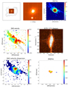 |
Fig. 3. 3C 076.1: FR I, 1″ = 0.64 kpc. Top left: radio contours (black) overlaid onto the MUSE optical continuum image in the 5800–6250 Å rest frame range. The size of the image is the whole MUSE field of view, 1′ × 1′. Top center: MUSE continuum image with superposed the region in which we explored the emission line properties (white square). Top right: [N II] emission line image extracted from the white square in the center panel. Surface brightness is 10−18 erg s−1 cm−2arcsec−2. Middle: velocity field from the [N II] line and position–velocity diagram extracted from the synthetic slit shown in the left panel (width 1″, PA = 50). Velocities are in units of km s−1. Bottom: velocity dispersion and [N II]/Hα ratio map. |
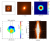 |
Fig. 4. 3C 078: FR I/LEG, 1″ = 0.56 kpc. Top left: radio contours (black) overlaid onto the MUSE optical continuum image. The size of the image is the whole MUSE field of view, 1′ × 1′. Top center: MUSE continuum image with superposed the region in which we explored the emission line properties (white square). Top right: [N II] emission line image extracted from the white square in the center panel. Surface brightness is 10−18 erg s−1 cm−2 arcsec−2. Bottom panels (left): velocity field (in km s−1) from the [N II] line; (right) position–velocity diagram extracted from the synthetic aperture shown in the left panel (width 0 |

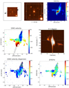 |
Fig. 5. 3C 079: FR II/HEG, 1″ = 4.0 kpc. Top left: radio contours (black) overlaid onto the MUSE continuum image. The size of the image is the whole MUSE field of view, 1′ × 1′. Top center: MUSE continuum image with superposed the region in which we explored the emission line properties (white square). Top right: [O III] emission line image extracted from the white square in the center panel. Surface brightness is 10−18 erg s−1 cm−2 arcsec−2. Central panels: (left) velocity field (in km s−1) from the [O III] line; (right) position–velocity diagram extracted from the synthetic aperture shown in the left panel. Bottom panels (left): velocity dispersion distribution (width 1″, PA = −20°) and (right) [O III]/Hα map. |
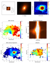 |
Fig. 6. 3C 088: FR II/LEG, 1″ = 0.60 kpc. Top left: radio contours (black) overlaid onto the MUSE continuum. The size of the image is the whole MUSE field of view, 1′ × 1′. Top center: MUSE continuum image with superposed the region in which we explored the emission line properties (white square). Top right: [N II] emission line image extracted from the white square in the center panel. Surface brightness is 10−18 erg s−1 cm−2 arcsec−2. Central panels: (left) velocity field (in km s−1) from the [N II] line; (right) position–velocity diagram extracted from the synthetic aperture shown in the left panel (width 0 |

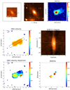 |
Fig. 7. 3C 089: FR I, 1″ = 2.46 kpc. Top left: radio contours (black) overlaid onto the MUSE continuum image. The size of the image is the whole MUSE field of view, 1′ × 1′. Top center: MUSE continuum image with superposed the region in which we explored the emission line properties (white square). Top right: [N II] emission line image extracted from the white square in the central panel. Surface brightness is 10−18 erg s−1 cm−2 arcsec−2. Central panels (left): velocity field (in km s−1) from the [N II] line; (right) position–velocity diagram extracted from the synthetic aperture shown in the left panel (width 1″, PA = 30°). Bottom panels (left): velocity dispersion distribution and (right) [N II]/Hα map. |
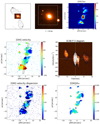 |
Fig. 8. 3C 098: FR II/HEG, 1″ = 0.60 kpc. Top left: radio contours (black) overlaid onto the MUSE continuum image. The size of the image is the whole MUSE field of view, 1′ × 1′. Top center: MUSE continuum image with superposed the region in which we explored the emission line properties (white square). Top right: [O III] emission line image extracted from the white square in the central panel. Surface brightness is 10−18 erg s−1 cm−2 arcsec−2. Central panels: (left) Velocity field (in km s−1) from the [O III] line; (right) position–velocity diagram extracted from the synthetic aperture shown in the left panel (width 1″, PA = −10°). Bottom panels (left): velocity dispersion distribution and (right) [O III]/Hα map. |
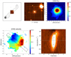 |
Fig. 9. 3C 105: FR II/HEG, 1″ = 1.67 kpc. Top left: radio contours (black) overlaid onto the MUSE continuum image. The size of the image is the whole MUSE field of view, 1′ × 1′. Top center: MUSE continuum image with superposed the region in which we explored the emission line properties (white square). Top right: [O III] emission line image extracted from the white square in the central panel. Surface brightness is 10−18erg s−1 cm−2arcsec−2. Bottom panels (left): velocity field (in km s−1) from the [O III] line (right) position–velocity diagram extracted from the synthetic aperture shown in the left panel (width 1″, PA = 50°). |
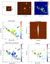 |
Fig. 10. 3C 135: FR II/HEG: 1″ = 2.26 kpc. Top left: radio contours (black) overlaid onto the MUSE continuum image. The size of the image is the whole MUSE field of view, 1′ × 1′. Top center: MUSE continuum image with superposed the region in which we explored the emission line properties (white square). Top right: [O III] emission line image extracted from the white square in the central panel. Surface brightness is 10−18 erg s−1 cm−2arcsec−2. Central panels: (left) velocity field (in km s−1) from the [O III] line; (right) position–velocity diagram extracted from the synthetic aperture shown in the left panel (width 1″, PA = 50°). Bottom panels (left): velocity dispersion distribution and (right) [O III]/Hα map. |
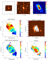 |
Fig. 11. 3C 180: FR II/HEG, 1″ = 3.58 kpc. Top left: radio contours (black) overlaid onto the MUSE continuum image. The size of the image is the whole MUSE field of view, 1′ × 1′. Top center: MUSE continuum imag e with superposed the region in which we explored the emission line properties (white square). Top right: [O III] emission line image extracted from the white square in the central panel. Surface brightness is 10−18 erg s−1 cm−2 arcsec−2. Central panels: (left) velocity field (in km s−1) from the [O III] line; (right) position–velocity diagram extracted from the synthetic aperture shown in the left panel (width 1″, PA = 40°). Bottom panels (left): velocity dispersion distribution and (right) [O III]/Hα map. |
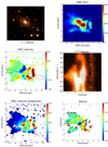 |
Fig. 12. 3C 196.1: FR II/LEG, 1″ = 3.30 kpc. Top left: radio contours (black) overlaid onto the MUSE continuum image. The size of the image is the whole MUSE field of view, 1′ × 1′. The white square marks the region in which we explored the emission line properties. Top right: [N II] emission line image extracted from the white square in the central panel. Surface brightness is 10−18 erg s−1 cm−2 arcsec−2. Central panels (left): velocity field (in km s−1) from the [N II] line; (right) position–velocity diagram extracted from the synthetic aperture shown in the left panel (width 1″, PA = 30°). Bottom panels (left): velocity dispersion distribution and (right) [N II]/Hα map. |
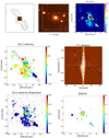 |
Fig. 13. 3C 198: FR II/SF, 1″ = 1.54 kpc. Top left: radio contours (black) overlaid onto the MUSE continuum image. The size of the image is the whole MUSE field of view, 1′ × 1′. Top center: MUSE continuum image with superposed the region in which we explored the emission line properties (white square). Top right: Hα emission line image extracted from the white square in the central panel. Surface brightness is 10−18 erg s−1 cm−2 arcsec−2. Central panels (left): velocity field (in km s−1) from the Hα line; (right) position–velocity diagram extracted from the synthetic aperture shown in the left panel (width 2″, PA = 30°). Bottom panels (left): velocity dispersion distribution and (right) [N II]/Hα map. |
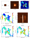 |
Fig. 14. 3C 227: FR II/BLO, 1″ = 1.62 kpc. Top left: radio contours (black) overlaid onto the MUSE continuum image. The size of the image is the whole MUSE field of view, 1′ × 1′. Top center: MUSE continuum image with superposed the region in which we explored the emission line properties (white square). Top right: [O III] emission line image extracted from the white square in the central panel. Surface brightness is 10−18erg s−1 cm−2 arcsec−2. Central panels (left): velocity field (in km s−1) from the [O III] line; (right) position–velocity diagram extracted from the synthetic aperture shown in the left panel (width 1″, PA = 50°). Bottom panels (left): velocity dispersion distribution and (right) [O III]/Hα map. |
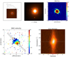 |
Fig. 15. 3C 264: FR I/LEG, 1″ = 0.43 kpc. Top left: radio contours (black) overlaid onto the MUSE continuum image. The size of the image is the whole MUSE field of view, 1′ × 1′. Top center: MUSE continuum image with superposed the region in which we explored the emission line properties (white square). Top right: [N II] emission line image extracted from the white square in the central panel. Surface brightness is 10−18 erg s−1 cm−2 arcsec−2. Bottom panels (left): velocity field (in km s−1) from the [N II] line; (right) position–velocity diagram extracted from the synthetic aperture shown in the left panel (width 0 |

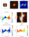 |
Fig. 16. 3C 272.1: FR I/LEG, 1″ = 0.06 kpc. Top left: radio contours (black) overlaid onto the MUSE continuum image. The size of the image is the whole MUSE field of view, 1′ × 1′. Top center: MUSE continuum image with superposed the region in which we explored the emission line properties (white square). Top right: [N II] emission line image extracted from the white square in the central panel. Surface brightness is 10−18 erg s−1 cm−2arcsec−2. Central panels (left): velocity field (in km s−1) from the [N II] line; (right) position–velocity diagram extracted from the synthetic aperture shown in the left panel (width 1″, PA = 80°). Bottom panels (left): velocity dispersion distribution and (right) [N II]/Hα map. |
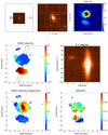 |
Fig. 17. 3C 287.1: FR II/BLO, 1″ = 3.53 kpc. Top left: radio contours (black) overlaid onto the MUSE continuum image. The size of the image is the whole MUSE field of view, 1′ × 1′. Top center: MUSE continuum image with superposed the region in which we explored the emission line properties (white square). Top right: [O III] emission line image extracted from the white square in the central panel. Surface brightness is 10−18 erg s−1 cm−2arcsec−2. Central panels: (left) velocity field (in km s−1) from the [O III] line; (right) position–velocity diagram extracted from the synthetic aperture shown in the left panel (width 1″, PA = −20°). Bottom panels (left): velocity dispersion distribution and (right) [O III]/Hα map. |
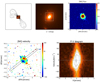 |
Fig. 18. 3C 296: FR I/LEG, 1″ = 0.49 kpc. Top left: radio contours (black) overlaid onto the MUSE continuum image. The size of the image is the whole MUSE field of view, 1′ × 1′. Top center: MUSE continuum image with superposed the region in which we explored the emission line properties (white square). Top right: [N II] emission line image extracted from the white square in the central panel. Surface brightness is 10−18 erg s−1 cm−2arcsec−2. Bottom panels (left): velocity field (in km s−1) from the [N II] line; (right) position–velocity diagram extracted from the synthetic aperture shown in the left panel (width 1″, PA = −50°). |
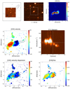 |
Fig. 19. 3C 300: FR II/HEG, 1″ = 4.17 kpc. Top left: radio contours (black) overlaid onto the MUSE continuum image. The size of the image is the whole MUSE field of view, 1′ × 1′. Top center: MUSE continuum image with superposed the region in which we explored the emission line properties (white square). Top right: [O III] emission line image extracted from the white square in the central panel. Surface brightness is 10−18 erg s−1 cm−2 arcsec−2. Central panels: (left) Velocity field (in km s−1) from the [O III] line; (right) position–velocity diagram extracted from the synthetic aperture shown in the left panel (width 1″, PA = −20°). Bottom panels (left): velocity dispersion distribution and (right) [O III]/Hα map. |
The emission line ratio maps provide important clues to the excitation mechanism of the gas. According to the location in the emission line ratio diagnostic plane defined by Kewley et al. (2006), we can separate Seyfert galaxies from starburst or LINER galaxies. In particular, assuming an intrinsic value of Ha/Hb of 3.1 (Ferland & Osterbrock 1985), a value of ([O III]/Hα) emission line ratio greater than ∼3 is indicative of a Seyfert-like nebular activity. Similarly, a [N II]/Hα value can be used instead to separate LINERs from starburst galaxies. We will investigate the spatially resolved emission line maps in comparison with the radio and X-ray emission in a future paper.
The definition of ordered rotation is based on the fit of the 2D gas velocity field obtained by using the kinemetry software (Krajnović et al. 2006) that reproduces the moments of the line-of-sight velocity distributions. The results from kinemetry obtained for all sources are presented in the Appendix.
3C 076.1. FR I, no optical classification, z = 0.032, 1″ = 0.64 kpc (see Fig. 3). Two diffuse emission line regions emerge from the compact central source, extending ∼4 kpc on each side. The central ELR shows regular rotation with an amplitude of ∼300 km s−1. The velocity dispersion is, except on the nucleus, consistent with the MUSE spectral resolution.
3C 078 (NGC 1218). FR I/LEG, z = 0.028, 1″ = 0.56 kpc (see Fig. 4). The central ELR is only marginally resolved.
3C 079. FR II/HEG, z = 0.256, 1″ = 4.0 kpc (see Fig. 5). The ELR has an X-shaped morphology. The two brightest and most extended structures (∼80 kpc of total size) are oriented perpendicularly to the radio axis, and show ordered rotation with an amplitude of ∼800 km s−1. In addition, there are several filaments of line emission of similar size but of lower brightness extending perpendicularly to the main emission line structure. The brightest regions of the ELR have higher [O III]/Hα values than those of lower brightness; no clear trend with distance is seen.
3C 088 (UGC 2748). FR II/LEG, z = 0.030, 1″ = 0.60 kpc (see Fig. 6). A diffuse halo of line emission, ∼3 kpc of radius, surrounds the central ELR. It shows significant rotation, with an amplitude of ∼170 km s−1. The velocity dispersion reaches ∼250 km s−1 on the nucleus but elsewhere is rather low. The [N II]/Hα ratio is higher in the central region than in the diffuse halo.
3C 089. FR I, no optical classification, z = 0.138, 1″ = 2.46 kpc (see Fig. 7). A linear feature of line emission emerges along the PA of the western radio jet and reaches a distance of ∼10 kpc. The velocity field is remarkably flat.
3C 098. FR II/HEG, z = 0.030, 1″ = 0.60 kpc (see Fig. 8). A series of bright knots extends on both sides of the nucleus to a distance of ∼15 kpc, oriented at PA ∼ −10°, ∼35° away from the radio axis. The velocity field is quite complex, but a general rotation is seen with the S side of the ELR receding from us and the N side approaching. The line wid th exceeds the instrumental value only in the central component of the ELR. The [O III]/Hα ratio has a radial structure, decreasing at larger angles from the radio axis, while no trend with distance is observed.
3C 105. FR II/HEG, z = 0.089, 1″ = 1.67 kpc (see Fig. 9). The ELR is compact, with a size of a few kpc. It shows rotation around PA ∼ 70° with an amplitude of ∼400 km s−1.
3C 135. FR II/HEG, z = 0.125, 1″ = 2.26 kpc (see Fig. 10). An irregular series of emission line knots form a conical structure, mainly toward the SW, reaching a distance of ∼77 kpc and tracing the edge of the western radio lobe. The ELR shows rapid rotation in the central regions, while the velocity gradients sharply decreases in the outer diffuse structures. The [O III]/Hα ratio shows a general decreasing trend toward larger radii.
3C 180. FR II/HEG, z = 0.220, 1″ = 3.58 kpc (see Fig. 11). A series of arc-like features is seen on both sides of the nucleus, confirming the structure already seen in the HST images (Baldi et al. 2019). The ELR extends by ∼45 kpc on both sides and it is oriented along a similar angle of the radio axis (the radio image used, the only available high resolution image from the NRAO VLA Archive Survey Images, is at a frequency of 8.4 GHz and only shows the two hot spots). In general, the ELR shows a rotating structure with a full amplitude of ∼700 km s−1, but with local velocity fluctuations on the larger scales. The velocity dispersion shows an increase at the edges of the brightest arcs. The [O III]/Hα has a complex structure.
3C 196.1. FR II/LEG, z = 0.198, 1″ = 3.30 kpc (see Fig. 12). Its radio structure is best seen in the 5 GHz image from Neff et al. (1995): it is a double source with a total size of 5″ (∼16 kpc) oriented along PA ∼ 40. The ELR has a similar size and orientation and its SW side enshrouds the radio lobe. In this region we detect very high recession velocities, exceeding ∼500 km s−1, and large line widths. These results suggest that we are seeing a cavity of ionized gas inflated by the radio outflow. The opposite NE side is more diffuse, with no significant velocity gradient and a small velocity dispersion. The SW line lobe has a higher [N II]/Hα than the opposite side.
3C 198. FR II/SF, z = 0.081, 1″ = 1.54 kpc (see Fig. 13). This is the only 3C source at z < 0.3 where the emission lines are dominated by the presence of star forming regions (Buttiglione et al. 2010). The ELR shows both compact knots and diffuse emission, mainly on its SW side where it reaches a distance of ∼45 kpc. While the bright knot on the E side is cospatial with a nearby galaxy, the remaining compact line features do not have continuum counterparts. All these structures have a spectrum characteristic of star formation, similarly to what is observed on the nucleus, suggestive of jet-induced star formation.
3C 227. FR II/BLO, z = 0.086, 1″ = 1.62 kpc (see Fig. 14). The ELR in this source covers the whole MUSE field of view, reaching distances of ∼50 kpc. It is dominated by a bright linear structure, oriented at PA ∼ 120°, showing evidence of ordered rotation out to a radius of ∼5″. A second structure of lower surface brightness gives an overall X-shaped structure to the ELR, similar to that seen in 3C 079. On the NE side this features wraps toward higher values of PA, and it also shows a large velocity gradient and a higher [O III]/Hα.
3C 258. As already mentioned above, we confirm that the identification of this radio source with a galaxy at redshift z = 0.165 is incorrect. We confirm the suggestion of Dey (1994) and Floyd et al. (2008) that it is instead a QSO at z ∼ 1.54, based on the presence of a single broad emission line λ = 7116 Å, likely Mg II at λ = 2798 Å in rest frame.
3C 264 (NGC 3862). FR I/LEG, z = 0.021, 1″ = 0.43 kpc (see Fig. 15). The central ELR is only marginally resolved, but it shows ordered rotation with an amplitude of ∼100 km s−1. A dusty disk or ring seen in HST data has been reported by Baum et al. (1997).
3C 272.1 (M 84). FR I/LEG, z = 0.003, 1″ = 0.068 kpc (see Fig. 16). This is the nearest source of our sample. The ELR extends for ∼2.5 kpc in the EW direction, perpendicular to the radio jets and cospatial with the dust lane crossing the nuclear regions (Martel et al. 1999). At the largest radii its linear structure opens in a fan-like shape, similarly to the dust distribution. It shows an ordered rotation with a full amplitude of ∼400 km s−1. The line width is always consistent with the MUSE instrumental resolution, except the central ∼2 ″, where it reaches ∼250 km s−1. There is a general trend of decreasing [N II]/Hα moving from E to W.
3C 287.1. FR II/BLO, z = 0.216, 1″ = 3.53 kpc (see Fig. 17). The central ELR is only marginally resolved. At a distance of ∼5″ toward the S, in a direction almost perpendicular to the radio jet, a detached diffuse ELR is also seen, with a large velocity offset of ∼400 km s−1 with respect to the nuclear component. The [O III]/Hα ratio has a complex structure. In particular the southern component of the ELR shows a strong gradient in [O III]/Hα.
3C 296 (NGC 5532). FR I/LEG, z = 0.024, 1″ = 0.49 kpc (see Fig. 18). The central ELR is only marginally resolved.
3C 300. FR II/HEG, z = 0.270, 1″ = 4.17 kpc (see Fig. 19). The ELR has an S-shaped structure extending ∼60 kpc in the EW direction and showing well-ordered rotation along its major axis. More diffuse emission is found on the N and W side out to radii of more than ∼60 kpc. The [O III]/Hα ratio is higher in the off-nuclear regions than in the center.
6. Summary and conclusions
We completed the presentation of the observations of the 37 RGs from the 3C catalog with redshift < 0.3 and declination < 20° obtained with the VLT/MUSE optical integral field spectroscoph by showing the results obtained for the second set of 17 sources; the first 20 were presented in Balmaverde et al. (2019). These data were obtained as part of the MURALES survey, a project whose aim is to explore the distribution and kinematics of the ionized gas in the most powerful radio sources in order to better understand the AGN feedback.
We presented the data analysis and, for each source, the resulting emission line images, the 2D gas velocity field, and an emission line ratio map indicative of the gas excitation origin. Thanks to their unprecedented depth these observations reveal ELRs extending several tens of kiloparsec in most objects.
All but 2 of the 26 FR IIs show large-scale structures of ionized gas with a median extent of 16 kpc, but reaching sizes ≳80 kpc. The central gas component is often (in 21 sources) quite regular and characteristic of rotation. On larger scales the gas kinematics is usually more complex. The gas excitation (derived from either [O III]/Hα or [N II]/Hα) shows a quite complex behavior. In some sources (e.g., 3C 300) it increases with distance, but the opposite behavior is also seen (e.g., 3C 088) and we also see objects in which no trend with distance is found (e.g., 3C 079). We also observed sources with a radial structure of the gas excitation, with higher ionization gas located along the radio axis (e.g., 3C 098 in this paper and 3C 033 in Paper II). This scenario suggests that different gas excitation mechanisms are concurrent in the various sources, and that the gas ionization status likely depends on many complex factors. We will investigate this issue in detail in a following paper.
There are no apparent differences between the ELR properties of the FR IIs of high and low gas excitation regarding luminosities or sizes. This is unexpected because it has been suggested that LEGs and HEGs are related to a different accretion process: hot versus cold gas (Baum et al. 1995; Hardcastle et al. 2007; Buttiglione et al. 2010). Nonetheless, in LEGs we detected large reservoirs of warm emitting line gas, similar in extent and luminosity to those found in HEGs. This finding leaves open the possibility that the two classes are connected in a evolutionary scenario, i.e., that a transition between HEGs and LEGs (or vice versa) occurs (see also Macconi et al. 2020).
Conversely, there is a clear connection between radio morphology, and in particular between the Fanaroff–Riley class and emission line properties. In the ten FR Is observed the line emission regions are generally compact, only a few kpc in size; only one case (3C 348) exceeds the size of the host reaching a radius of ∼40 kpc. The ELRs in FR Is are smaller and less luminous than those seen in the FR IIs. This deficit is found even comparing sources at the same level of line nuclear luminosity, a robust proxy for the strength of the nuclear ionizing continuum. This implies that what distinguishes objects belonging to the two radio morphological classes is a different content of gas in the warm or cold phase on scales larger than the host galaxy, the FR Is being generally gas poor. This result adds to similar conclusions obtained from the properties of the interstellar medium of RGs (see, e.g., de Koff et al. 2000; Ocaña Flaquer et al. 2010).
We also confirmed that the optical identification of 3C 258 is incorrect. The currently identified optical counterpart is offset by 2 8 with respect to the compact radio source. Conversely, at the location of the radio emission both the HST and Chandra images show the presence of a point-like object. The MUSE spectrum of this object shows a single emission line, with a broad profile, at λ = 7116 Å, the most likely identification of this line being Mg II at λ2798 Å. This indicates an association with a type I AGN at a tentative redshift z ∼ 1.54.
As already discussed in the Introduction, AGN feedback in radio-loud sources can manifest itself in two different ways: radio and radiative modes. They correspond to a transfer of energy to the ambient medium from the relativistic jets and from nuclear outflows, respectively. In two companion papers we will address in detail these issues by studying the origin of the extended emission line structures, and in particular their connection with the radio emission, and we will explore the properties of nuclear outflows of ionized gas.
Acknowledgments
This research has made use of the NASA/IPAC Extragalactic Database (NED), which is operated by the Jet Propulsion Laboratory, California Institute of Technology, under contract with the National Aeronautics and Space Administration. The radio images were produced as part of the NRAO VLA Archive Survey, (c) AUI/NRAO. The NVAS can be browsed through http://archive.nrao.edu/nvas/. S. Baum and C. O’Dea are grateful to the Natural Sciences and Engineering Research Council (NSERC) of Canada. We thank the anonymous referee for her/his useful comments and suggestions.
References
- Bacon, R., Accardo, M., Adjali, L., et al. 2010, Proc. SPIE, 7735, 773508 [Google Scholar]
- Baldi, R. D., Capetti, A., Buttiglione, S., Chiaberge, M., & Celotti, A. 2013, A&A, 560, A81 [NASA ADS] [CrossRef] [EDP Sciences] [Google Scholar]
- Baldi, R. D., Rodríguez Zaurín, J., Chiaberge, M., et al. 2019, ApJ, 870, 53 [NASA ADS] [CrossRef] [Google Scholar]
- Balmaverde, B., Marconi, A., Brusa, M., et al. 2016, A&A, 585, A148 [NASA ADS] [CrossRef] [EDP Sciences] [Google Scholar]
- Balmaverde, B., Capetti, A., Marconi, A., & Venturi, G. 2018a, A&A, 612, A19 [NASA ADS] [CrossRef] [EDP Sciences] [Google Scholar]
- Balmaverde, B., Capetti, A., Marconi, A., et al. 2018b, A&A, 619, A83 [NASA ADS] [CrossRef] [EDP Sciences] [Google Scholar]
- Balmaverde, B., Capetti, A., Marconi, A., et al. 2019, A&A, 632, A124 [CrossRef] [EDP Sciences] [Google Scholar]
- Baum, S. A., & Heckman, T. 1989a, ApJ, 336, 681 [NASA ADS] [CrossRef] [Google Scholar]
- Baum, S. A., & Heckman, T. 1989b, ApJ, 336, 702 [NASA ADS] [CrossRef] [Google Scholar]
- Baum, S. A., Zirbel, E. L., & O’Dea, C. P. 1995, ApJ, 451, 88 [NASA ADS] [CrossRef] [Google Scholar]
- Baum, S. A., O’Dea, C. P., Giovannini, G., et al. 1997, ApJ, 483, 178 [NASA ADS] [CrossRef] [Google Scholar]
- Baum, S. A., Gallimore, J. F., O’Dea, C. P., et al. 2010, ApJ, 710, 289 [NASA ADS] [CrossRef] [Google Scholar]
- Bennert, N., Falcke, H., Schulz, H., Wilson, A. S., & Wills, B. J. 2002, ApJ, 574, L105 [NASA ADS] [CrossRef] [Google Scholar]
- Bennett, C. L., Larson, D., Weiland, J. L., & Hinshaw, G. 2014, ApJ, 794, 135 [NASA ADS] [CrossRef] [Google Scholar]
- Bîrzan, L., Rafferty, D. A., McNamara, B. R., Wise, M. W., & Nulsen, P. E. J. 2004, ApJ, 607, 800 [NASA ADS] [CrossRef] [Google Scholar]
- Bîrzan, L., Rafferty, D. A., Brüggen, M., et al. 2020, MNRAS, 496, 2613 [CrossRef] [Google Scholar]
- Blanton, E. L., Randall, S. W., Clarke, T. E., et al. 2011, ApJ, 737, 99 [NASA ADS] [CrossRef] [Google Scholar]
- Buttiglione, S., Capetti, A., Celotti, A., et al. 2009, A&A, 495, 1033 [NASA ADS] [CrossRef] [EDP Sciences] [Google Scholar]
- Buttiglione, S., Capetti, A., Celotti, A., et al. 2010, A&A, 509, A6 [NASA ADS] [CrossRef] [EDP Sciences] [Google Scholar]
- Buttiglione, S., Capetti, A., Celotti, A., et al. 2011, A&A, 525, A28 [NASA ADS] [CrossRef] [EDP Sciences] [Google Scholar]
- Cappellari, M. 2017, MNRAS, 466, 798 [NASA ADS] [CrossRef] [Google Scholar]
- Cappellari, M., & Copin, Y. 2003, MNRAS, 342, 345 [NASA ADS] [CrossRef] [Google Scholar]
- Carniani, S., Marconi, A., Maiolino, R., et al. 2016, A&A, 591, A28 [NASA ADS] [CrossRef] [EDP Sciences] [Google Scholar]
- Chen, J., Shi, Y., Dempsey, R., et al. 2019, MNRAS, 489, 855 [CrossRef] [Google Scholar]
- Cresci, G., & Maiolino, R. 2018, Nat. Astron., 2, 179 [NASA ADS] [CrossRef] [Google Scholar]
- de Koff, S., Baum, S. A., Sparks, W. B., et al. 1996, ApJS, 107, 621 [NASA ADS] [CrossRef] [Google Scholar]
- de Koff, S., Best, P., Baum, S. A., et al. 2000, ApJS, 129, 33 [NASA ADS] [CrossRef] [Google Scholar]
- Dey, A. 1994, Ph.D. Thesis, AA (University of Californina, Berkeley) [Google Scholar]
- Fabian, A. C. 2012, ARA&A, 50, 455 [Google Scholar]
- Fanaroff, B. L., & Riley, J. M. 1974, MNRAS, 167, 31P [Google Scholar]
- Ferland, G. J., & Osterbrock, D. E. 1985, ApJ, 289, 105 [CrossRef] [Google Scholar]
- Floyd, D. J. E., Axon, D., Baum, S., et al. 2008, ApJS, 177, 148 [NASA ADS] [CrossRef] [Google Scholar]
- Hardcastle, M. J., Evans, D. A., & Croston, J. H. 2007, MNRAS, 376, 1849 [NASA ADS] [CrossRef] [Google Scholar]
- Hine, R. G., & Longair, M. S. 1979, MNRAS, 188, 111 [NASA ADS] [Google Scholar]
- Husemann, B., Jahnke, K., Sánchez, S. F., et al. 2014, MNRAS, 443, 755 [NASA ADS] [CrossRef] [Google Scholar]
- Kewley, L. J., Groves, B., Kauffmann, G., & Heckman, T. 2006, MNRAS, 372, 961 [NASA ADS] [CrossRef] [Google Scholar]
- Krajnović, D., Cappellari, M., de Zeeuw, P. T., & Copin, Y. 2006, MNRAS, 366, 787 [NASA ADS] [CrossRef] [Google Scholar]
- Laing, R. A., Jenkins, C. R., Wall, J. V., & Unger, S. W. 1994, in The Physics of Active Galaxies, eds. G. V. Bicknell, M. A. Dopita, & P. J. Quinn, ASP Conf. Ser., 54, 201 [Google Scholar]
- Macconi, D., Torresi, E., Grandi, P., Boccardi, B., & Vignali, C. 2020, MNRAS, 493, 4355 [CrossRef] [Google Scholar]
- Martel, A. R., Baum, S. A., Sparks, W. B., et al. 1999, ApJS, 122, 81 [NASA ADS] [CrossRef] [Google Scholar]
- Massaro, F., D’Abrusco, R., Tosti, G., et al. 2012, ApJ, 750, 138 [NASA ADS] [CrossRef] [Google Scholar]
- McNamara, B. R., & Nulsen, P. E. J. 2007, ARA&A, 45, 117 [NASA ADS] [CrossRef] [MathSciNet] [Google Scholar]
- Mulchaey, J. S., Wilson, A. S., & Tsvetanov, Z. 1996, ApJ, 467, 197 [NASA ADS] [CrossRef] [Google Scholar]
- Neff, S. G., Roberts, L., & Hutchings, J. B. 1995, ApJS, 99, 349 [NASA ADS] [CrossRef] [Google Scholar]
- Ocaña Flaquer, B., Leon, S., Combes, F., & Lim, J. 2010, A&A, 518, A9 [NASA ADS] [CrossRef] [EDP Sciences] [Google Scholar]
- Panagoulia, E. K., Fabian, A. C., Sanders, J. S., & Hlavacek-Larrondo, J. 2014, MNRAS, 444, 1236 [NASA ADS] [CrossRef] [Google Scholar]
- Privon, G. C., O’Dea, C. P., Baum, S. A., et al. 2008, ApJS, 175, 423 [NASA ADS] [CrossRef] [Google Scholar]
- Rawlings, S., & Saunders, R. 1991, Nature, 349, 138 [NASA ADS] [CrossRef] [Google Scholar]
- Rawlings, S., Saunders, R., Eales, S. A., & Mackay, C. D. 1989, MNRAS, 240, 701 [NASA ADS] [Google Scholar]
- Richstone, D. O., & Oke, J. B. 1977, ApJ, 213, 8 [NASA ADS] [CrossRef] [Google Scholar]
- Spinrad, H., Marr, J., Aguilar, L., & Djorgovski, S. 1985, PASP, 97, 932 [NASA ADS] [CrossRef] [Google Scholar]
- Stockton, A. 1976, ApJ, 205, L113 [NASA ADS] [CrossRef] [Google Scholar]
- Sun, A.-L., Greene, J. E., Zakamska, N. L., et al. 2018, MNRAS, 480, 2302 [NASA ADS] [CrossRef] [Google Scholar]
- Tremblay, G. R., Chiaberge, M., Sparks, W. B., et al. 2009, ApJS, 183, 278 [NASA ADS] [CrossRef] [Google Scholar]
- Wampler, E. J., Robinson, L. B., Burbidge, E. M., & Baldwin, J. A. 1975, ApJ, 198, L49 [NASA ADS] [CrossRef] [Google Scholar]
- Weilbacher, P. M., Palsa, R., Streicher, O., et al. 2020, A&A, 641, A28 [CrossRef] [EDP Sciences] [Google Scholar]
- Wylezalek, D., & Zakamska, N. L. 2016, MNRAS, 461, 3724 [NASA ADS] [CrossRef] [Google Scholar]
- Wyndham, J. D. 1966, ApJ, 144, 459 [CrossRef] [Google Scholar]
Appendix A: Analysis of the gas kinematics
We fit the 2D gas velocity field in the innermost regions with the kinemetry software (Krajnović et al. 2006), a generalization of surface photometry that reproduces the moments of the line-of-sight velocity distributions. The parameters of interest to us returned by this software are (1) the kinematical PA, (2) the coefficient of the harmonic expansion k1 (from which the rotation curve is derived), and (3) the ratio of the fifth to the first coefficient k5/k1 and its error σk5/k1 (which quantifies the deviations from purely ordered rotation). In this Appendix we show the results obtained for all sources, excluding only 3C 089 where the velocity field is remarkably flat.
We considered that a source shows ordered rotation when the kinematical parameters are defined at a radius larger than 2 times the seeing of the observations and where (k5/k1 + σk5/k1) < 0.2.
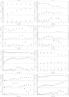 |
Fig. A.1. Results obtained for 36 radio galaxies (all but 3C 089) with the kinemetry software. From top to bottom in each panel: kinematic position angle PA (in degrees), amplitude of the rotation curve (in km s−1), and the ratio of the fifth to the first coefficient k5/k1, which quantifies the deviations from simple rotation. |
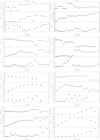 |
Fig. A.1. continued. |
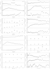 |
Fig. A.1. continued. |
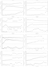 |
Fig. A.1. continued. |
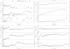 |
Fig. A.1. continued. |
All Tables
Main properties of the 3C subsample observed with MUSE, and the observations log.
All Figures
|
Fig. 1. Radio contours (white) of 3C 258 from Neff et al. (1995) superimposed on the optical continuum image (field of view 25″ × 25″) derived from the MUSE data. The radio source is offset by |
| In the text | |
|
Fig. 2. From top to bottom, first and second panels: logarithm of the luminosities of the extended ELRs in the [N II] line vs. nuclear line luminosity and radio luminosities (all quantities in erg s−1). Sources are coded with symbols combining the optical spectroscopic classification and radio morphology. The dashed line is the bisectrix of the plane. Third panel: luminosity of the Hα+[N II] emission line vs. redshift. Fourth panel: logarithm of the size of the extended ELR (in kpc) vs. nuclear line luminosity. The dashed line shows the |
| In the text | |
|
Fig. 3. 3C 076.1: FR I, 1″ = 0.64 kpc. Top left: radio contours (black) overlaid onto the MUSE optical continuum image in the 5800–6250 Å rest frame range. The size of the image is the whole MUSE field of view, 1′ × 1′. Top center: MUSE continuum image with superposed the region in which we explored the emission line properties (white square). Top right: [N II] emission line image extracted from the white square in the center panel. Surface brightness is 10−18 erg s−1 cm−2arcsec−2. Middle: velocity field from the [N II] line and position–velocity diagram extracted from the synthetic slit shown in the left panel (width 1″, PA = 50). Velocities are in units of km s−1. Bottom: velocity dispersion and [N II]/Hα ratio map. |
| In the text | |
|
Fig. 4. 3C 078: FR I/LEG, 1″ = 0.56 kpc. Top left: radio contours (black) overlaid onto the MUSE optical continuum image. The size of the image is the whole MUSE field of view, 1′ × 1′. Top center: MUSE continuum image with superposed the region in which we explored the emission line properties (white square). Top right: [N II] emission line image extracted from the white square in the center panel. Surface brightness is 10−18 erg s−1 cm−2 arcsec−2. Bottom panels (left): velocity field (in km s−1) from the [N II] line; (right) position–velocity diagram extracted from the synthetic aperture shown in the left panel (width 0 |
| In the text | |
|
Fig. 5. 3C 079: FR II/HEG, 1″ = 4.0 kpc. Top left: radio contours (black) overlaid onto the MUSE continuum image. The size of the image is the whole MUSE field of view, 1′ × 1′. Top center: MUSE continuum image with superposed the region in which we explored the emission line properties (white square). Top right: [O III] emission line image extracted from the white square in the center panel. Surface brightness is 10−18 erg s−1 cm−2 arcsec−2. Central panels: (left) velocity field (in km s−1) from the [O III] line; (right) position–velocity diagram extracted from the synthetic aperture shown in the left panel. Bottom panels (left): velocity dispersion distribution (width 1″, PA = −20°) and (right) [O III]/Hα map. |
| In the text | |
|
Fig. 6. 3C 088: FR II/LEG, 1″ = 0.60 kpc. Top left: radio contours (black) overlaid onto the MUSE continuum. The size of the image is the whole MUSE field of view, 1′ × 1′. Top center: MUSE continuum image with superposed the region in which we explored the emission line properties (white square). Top right: [N II] emission line image extracted from the white square in the center panel. Surface brightness is 10−18 erg s−1 cm−2 arcsec−2. Central panels: (left) velocity field (in km s−1) from the [N II] line; (right) position–velocity diagram extracted from the synthetic aperture shown in the left panel (width 0 |
| In the text | |
|
Fig. 7. 3C 089: FR I, 1″ = 2.46 kpc. Top left: radio contours (black) overlaid onto the MUSE continuum image. The size of the image is the whole MUSE field of view, 1′ × 1′. Top center: MUSE continuum image with superposed the region in which we explored the emission line properties (white square). Top right: [N II] emission line image extracted from the white square in the central panel. Surface brightness is 10−18 erg s−1 cm−2 arcsec−2. Central panels (left): velocity field (in km s−1) from the [N II] line; (right) position–velocity diagram extracted from the synthetic aperture shown in the left panel (width 1″, PA = 30°). Bottom panels (left): velocity dispersion distribution and (right) [N II]/Hα map. |
| In the text | |
|
Fig. 8. 3C 098: FR II/HEG, 1″ = 0.60 kpc. Top left: radio contours (black) overlaid onto the MUSE continuum image. The size of the image is the whole MUSE field of view, 1′ × 1′. Top center: MUSE continuum image with superposed the region in which we explored the emission line properties (white square). Top right: [O III] emission line image extracted from the white square in the central panel. Surface brightness is 10−18 erg s−1 cm−2 arcsec−2. Central panels: (left) Velocity field (in km s−1) from the [O III] line; (right) position–velocity diagram extracted from the synthetic aperture shown in the left panel (width 1″, PA = −10°). Bottom panels (left): velocity dispersion distribution and (right) [O III]/Hα map. |
| In the text | |
|
Fig. 9. 3C 105: FR II/HEG, 1″ = 1.67 kpc. Top left: radio contours (black) overlaid onto the MUSE continuum image. The size of the image is the whole MUSE field of view, 1′ × 1′. Top center: MUSE continuum image with superposed the region in which we explored the emission line properties (white square). Top right: [O III] emission line image extracted from the white square in the central panel. Surface brightness is 10−18erg s−1 cm−2arcsec−2. Bottom panels (left): velocity field (in km s−1) from the [O III] line (right) position–velocity diagram extracted from the synthetic aperture shown in the left panel (width 1″, PA = 50°). |
| In the text | |
|
Fig. 10. 3C 135: FR II/HEG: 1″ = 2.26 kpc. Top left: radio contours (black) overlaid onto the MUSE continuum image. The size of the image is the whole MUSE field of view, 1′ × 1′. Top center: MUSE continuum image with superposed the region in which we explored the emission line properties (white square). Top right: [O III] emission line image extracted from the white square in the central panel. Surface brightness is 10−18 erg s−1 cm−2arcsec−2. Central panels: (left) velocity field (in km s−1) from the [O III] line; (right) position–velocity diagram extracted from the synthetic aperture shown in the left panel (width 1″, PA = 50°). Bottom panels (left): velocity dispersion distribution and (right) [O III]/Hα map. |
| In the text | |
|
Fig. 11. 3C 180: FR II/HEG, 1″ = 3.58 kpc. Top left: radio contours (black) overlaid onto the MUSE continuum image. The size of the image is the whole MUSE field of view, 1′ × 1′. Top center: MUSE continuum imag e with superposed the region in which we explored the emission line properties (white square). Top right: [O III] emission line image extracted from the white square in the central panel. Surface brightness is 10−18 erg s−1 cm−2 arcsec−2. Central panels: (left) velocity field (in km s−1) from the [O III] line; (right) position–velocity diagram extracted from the synthetic aperture shown in the left panel (width 1″, PA = 40°). Bottom panels (left): velocity dispersion distribution and (right) [O III]/Hα map. |
| In the text | |
|
Fig. 12. 3C 196.1: FR II/LEG, 1″ = 3.30 kpc. Top left: radio contours (black) overlaid onto the MUSE continuum image. The size of the image is the whole MUSE field of view, 1′ × 1′. The white square marks the region in which we explored the emission line properties. Top right: [N II] emission line image extracted from the white square in the central panel. Surface brightness is 10−18 erg s−1 cm−2 arcsec−2. Central panels (left): velocity field (in km s−1) from the [N II] line; (right) position–velocity diagram extracted from the synthetic aperture shown in the left panel (width 1″, PA = 30°). Bottom panels (left): velocity dispersion distribution and (right) [N II]/Hα map. |
| In the text | |
|
Fig. 13. 3C 198: FR II/SF, 1″ = 1.54 kpc. Top left: radio contours (black) overlaid onto the MUSE continuum image. The size of the image is the whole MUSE field of view, 1′ × 1′. Top center: MUSE continuum image with superposed the region in which we explored the emission line properties (white square). Top right: Hα emission line image extracted from the white square in the central panel. Surface brightness is 10−18 erg s−1 cm−2 arcsec−2. Central panels (left): velocity field (in km s−1) from the Hα line; (right) position–velocity diagram extracted from the synthetic aperture shown in the left panel (width 2″, PA = 30°). Bottom panels (left): velocity dispersion distribution and (right) [N II]/Hα map. |
| In the text | |
|
Fig. 14. 3C 227: FR II/BLO, 1″ = 1.62 kpc. Top left: radio contours (black) overlaid onto the MUSE continuum image. The size of the image is the whole MUSE field of view, 1′ × 1′. Top center: MUSE continuum image with superposed the region in which we explored the emission line properties (white square). Top right: [O III] emission line image extracted from the white square in the central panel. Surface brightness is 10−18erg s−1 cm−2 arcsec−2. Central panels (left): velocity field (in km s−1) from the [O III] line; (right) position–velocity diagram extracted from the synthetic aperture shown in the left panel (width 1″, PA = 50°). Bottom panels (left): velocity dispersion distribution and (right) [O III]/Hα map. |
| In the text | |
|
Fig. 15. 3C 264: FR I/LEG, 1″ = 0.43 kpc. Top left: radio contours (black) overlaid onto the MUSE continuum image. The size of the image is the whole MUSE field of view, 1′ × 1′. Top center: MUSE continuum image with superposed the region in which we explored the emission line properties (white square). Top right: [N II] emission line image extracted from the white square in the central panel. Surface brightness is 10−18 erg s−1 cm−2 arcsec−2. Bottom panels (left): velocity field (in km s−1) from the [N II] line; (right) position–velocity diagram extracted from the synthetic aperture shown in the left panel (width 0 |
| In the text | |
|
Fig. 16. 3C 272.1: FR I/LEG, 1″ = 0.06 kpc. Top left: radio contours (black) overlaid onto the MUSE continuum image. The size of the image is the whole MUSE field of view, 1′ × 1′. Top center: MUSE continuum image with superposed the region in which we explored the emission line properties (white square). Top right: [N II] emission line image extracted from the white square in the central panel. Surface brightness is 10−18 erg s−1 cm−2arcsec−2. Central panels (left): velocity field (in km s−1) from the [N II] line; (right) position–velocity diagram extracted from the synthetic aperture shown in the left panel (width 1″, PA = 80°). Bottom panels (left): velocity dispersion distribution and (right) [N II]/Hα map. |
| In the text | |
|
Fig. 17. 3C 287.1: FR II/BLO, 1″ = 3.53 kpc. Top left: radio contours (black) overlaid onto the MUSE continuum image. The size of the image is the whole MUSE field of view, 1′ × 1′. Top center: MUSE continuum image with superposed the region in which we explored the emission line properties (white square). Top right: [O III] emission line image extracted from the white square in the central panel. Surface brightness is 10−18 erg s−1 cm−2arcsec−2. Central panels: (left) velocity field (in km s−1) from the [O III] line; (right) position–velocity diagram extracted from the synthetic aperture shown in the left panel (width 1″, PA = −20°). Bottom panels (left): velocity dispersion distribution and (right) [O III]/Hα map. |
| In the text | |
|
Fig. 18. 3C 296: FR I/LEG, 1″ = 0.49 kpc. Top left: radio contours (black) overlaid onto the MUSE continuum image. The size of the image is the whole MUSE field of view, 1′ × 1′. Top center: MUSE continuum image with superposed the region in which we explored the emission line properties (white square). Top right: [N II] emission line image extracted from the white square in the central panel. Surface brightness is 10−18 erg s−1 cm−2arcsec−2. Bottom panels (left): velocity field (in km s−1) from the [N II] line; (right) position–velocity diagram extracted from the synthetic aperture shown in the left panel (width 1″, PA = −50°). |
| In the text | |
|
Fig. 19. 3C 300: FR II/HEG, 1″ = 4.17 kpc. Top left: radio contours (black) overlaid onto the MUSE continuum image. The size of the image is the whole MUSE field of view, 1′ × 1′. Top center: MUSE continuum image with superposed the region in which we explored the emission line properties (white square). Top right: [O III] emission line image extracted from the white square in the central panel. Surface brightness is 10−18 erg s−1 cm−2 arcsec−2. Central panels: (left) Velocity field (in km s−1) from the [O III] line; (right) position–velocity diagram extracted from the synthetic aperture shown in the left panel (width 1″, PA = −20°). Bottom panels (left): velocity dispersion distribution and (right) [O III]/Hα map. |
| In the text | |
|
Fig. A.1. Results obtained for 36 radio galaxies (all but 3C 089) with the kinemetry software. From top to bottom in each panel: kinematic position angle PA (in degrees), amplitude of the rotation curve (in km s−1), and the ratio of the fifth to the first coefficient k5/k1, which quantifies the deviations from simple rotation. |
| In the text | |
|
Fig. A.1. continued. |
| In the text | |
|
Fig. A.1. continued. |
| In the text | |
|
Fig. A.1. continued. |
| In the text | |
|
Fig. A.1. continued. |
| In the text | |
Current usage metrics show cumulative count of Article Views (full-text article views including HTML views, PDF and ePub downloads, according to the available data) and Abstracts Views on Vision4Press platform.
Data correspond to usage on the plateform after 2015. The current usage metrics is available 48-96 hours after online publication and is updated daily on week days.
Initial download of the metrics may take a while.