| Issue |
A&A
Volume 645, January 2021
|
|
|---|---|---|
| Article Number | A71 | |
| Number of page(s) | 19 | |
| Section | Planets and planetary systems | |
| DOI | https://doi.org/10.1051/0004-6361/202039042 | |
| Published online | 15 January 2021 | |
The GAPS Programme at TNG
XXVIII. A pair of hot-Neptunes orbiting the young star TOI-942★,★★
1
Astronomy Department and Van Vleck Observatory, Wesleyan University,
Middletown,
CT 06459, USA
e-mail: icarleo@wesleyan.edu
2
INAF – Osservatorio Astronomico di Padova,
Vicolo dell’Osservatorio 5,
35122
Padova, Italy
3
Aix Marseille Univ, CNRS, CNES, LAM,
Marseille,
France
4
Dipartimento di Fisica e Astronomia Galileo Galilei, Universitá di Padova,
Vicolo dellOsservatorio 3,
35122
Padova, Italy
5
INAF – Osservatorio Astrofisico di Catania,
Via S. Sofia 78,
95123
Catania, Italy
6
Department of Astronomy, University of Tokyo,
7-3-1 Hongo,
Bunkyo-ku,
Tokyo 113-0033, Japan
7
INAF – Osservatorio Astronomico di Palermo,
Piazza del Parlamento, 1,
90134 Palermo, Italy
8
Institute for Space Astrophysics and Planetology INAF-IAPS Via Fosso del Cavaliere 100,
00133 Roma, Italy
9
INAF – Osservatorio Astronomico di Brera,
Via E. Bianchi 46,
23807 Merate, Italy
10
INAF – Osservatorio Astrofisico di Torino,
Via Osservatorio 20,
10025
Pino Torinese, Italy
11
INAF – Osservatorio Astrofisico di Arcetri,
Largo Enrico Fermi 5,
50125 Firenze, Italy
12
ETH Zürich, Institute for Particle Physics and Astrophysics,
Wolfgang-Pauli-Str. 27,
8093 Zürich, Switzerland
13
INAF – Osservatorio Astronomico di Trieste,
Via Tiepolo 11,
34143 Trieste, Italy
14
Fundación Galileo Galilei-INAF,
Rambla José Ana Fernandez Pérez 7,
38712 Breña Baja,
TF, Spain
15
INAF – Osservatorio Astronomico di Capodimonte,
Salita Moiariello 16,
80131 Napoli, Italy
16
Thüringer Landessternwarte Tautenburg,
Sternwarte 5,
07778 Tautenberg, Germany
17
Dipartimento di Fisica G. Occhialini, Università degli Studi di Milano-Bicocca,
Piazza della Scienza 3,
20126 Milano, Italy
18
Leibniz-Institut für Astrophysik Potsdam (AIP),
An der Sternwarte 16,
14482 Potsdam, Germany
19
Department of Physics, University of Rome “Tor Vergata”,
Via della Ricerca Scientifica 1,
00133
Rome, Italy
20
Max Planck Institute for Astronomy,
Königstuhl 17,
69117
Heidelberg, Germany
21
INAF – Osservatorio Astronomico di Cagliari & REM,
Via della Scienza, 5,
09047 Selargius CA, Italy
Received:
27
July
2020
Accepted:
25
November
2020
Context. Young stars and multi-planet systems are two types of primary objects that allow us to study, understand, and constrain planetary formation and evolution theories.
Aims. We validate the physical nature of two Neptune-sized planets transiting TOI-942 (TYC 5909-319-1), a previously unacknowledged young star (50−20+30 Myr) observed by the TESS space mission in Sector 5.
Methods. Thanks to a comprehensive stellar characterization, TESS light curve modeling and precise radial-velocity measurements, we validated the planetary nature of the TESS candidate and detected an additional transiting planet in the system on a larger orbit.
Results. From photometric and spectroscopic observations we performed an exhaustive stellar characterization and derived the main stellar parameters. TOI-942 is a relatively active K2.5V star (log R′HK = −4.17 ± 0.01) with rotation period Prot = 3.39 ± 0.01 days, a projected rotation velocity v sin i⋆ = 13.8 ± 0.5 km s−1, and a radius of ~0.9 R⊙. We found that the inner planet, TOI-942 b, has an orbital period Pb = 4.3263 ± 0.0011 days, a radius Rb = 4.242−0.313+0.376 R⊕, and a mass upper limit of 16 M⊕ at 1σ confidence level. The outer planet, TOI-942 c, has an orbital period Pc = 10.1605−0.0053+0.0056 days, a radius Rc = 4.793−0.351+0.410 R⊕, and a mass upper limit of 37 M⊕ at 1σ confidence level.
Key words: planetary systems / techniques: photometric / techniques: spectroscopic / stars: fundamental parameters / techniques: radial velocities
Based on observations made with the Italian Telescopio Nazionale Galileo (TNG) operated by the Fundación Galileo Galilei (FGG) of the Istituto Nazionale di Astrofisica (INAF) at the Observatorio del Roque de los Muchachos (La Palma, Canary Islands, Spain).
The authors became aware of a parallel effort on the characterization of TOI-942 by Zhou et al. (2021) in the late stages of the manuscript preparations. The submissions are coordinated, and no analyses or results were shared prior to submission.
© ESO 2021
1 Introduction
The Kepler mission (Borucki et al. 2010) discovered hundreds of multi-planet systems (Weiss et al. 2018), enabling detailed statistical studies; it is now the Transiting Exoplanet Survey Satellite (TESS; Ricker et al. 2014) that is allowing us to add dozens of confirmed planets to the sample and ~2300 candidates1, among which several multi-planet systems (e.g., Huang et al. 2018; Quinn et al. 2019; Günther et al. 2019; Gandolfi et al. 2019; Crossfield et al. 2019; Carleo et al. 2020a; Gilbert et al. 2020; Nowak et al. 2020). Studying the properties of multi-planet systems, such as orbital periods, obliquities and eccentricities, planetary radii, as well as the chemistry of exoplanetary atmospheres and their hydrodynamical evolution, is essential to better constrain the planetary formation and evolution theories.
It is now clear that many exoplanetary systems do not follow the same architecture as the Solar System. Instead, they show an extraordinary diversity, which makes it difficult to adopt a single formation scenario for all the observed systems. Multi-planet systems represent an excellent opportunity to study and compare the observable properties of the exoplanets orbiting the same star and formed under the same initial conditions.
Planetary systems at young ages are valuable resources that can help us to understand formation and migration processes, the physical evolution of the planet themselves (e.g., gravitational contraction), and the planet evaporation under high-energy irradiation. To date, TESS has revealed a two-planet system HD 63433, which is a member of the ~400 Myr old Ursa Major association (Mann et al. 2020); single planets around the 40–45 Myr old star DS Tuc (Benatti et al. 2019; Newton et al. 2019); the ~20 Myr old star AU Mic (Plavchan et al. 2020); and the 10–20 Myr old star HIP 67522 (Rizzuto et al. 2020). The K2 mission has also contributed significantly to this field with the discovery of the youngest multi-planet system with transiting planets known to date (the four-planet system around the 23 Myr old star V1298 Tau, David et al. 2019) and the youngest single transiting planet (K2-33 at an age of 5–10 Myr, David et al. 2016). Several single and multi-planet systems were also identified in the Hyades and Praesepe open clusters (e.g., Malavolta et al. 2016; Rizzuto et al. 2017).
In this paper we report on the validation of a Neptune-sized planet and the discovery of an additional super-Neptune planetary companion, both transiting TOI-942, an active K2.5V star observed by TESS in Sector 5. With an age of  Myr, this is the youngest multi-planet system identified by TESS so far. The star was not previously thought to be a young object, but it was selected as a promising case of a young planet-host candidate from our systematic check of stellar properties of the TESS Objects of Interest (TOI)2. The presence of X-ray emission from ROSAT and high levels of activity from RAVE (Žerjal et al. 2017) alerted us to its possible youth, which was confirmed by the detailed analysis of the TESS light curve and the first spectrum acquired with HARPS-N at TNG. We then started the radial velocity (RV) follow-up in order to confirm the planet candidate as part of the Global Architecture of Planetary Systems (GAPS) Young Objects Project (Carleo et al. 2020b).
The paper is organized as follows. We first describe the observations of TOI-942, including TESS photometry, ground-based photometry, and spectroscopy in Sects. 2.1, 2.2, and 2.3, respectively. We perform a comprehensive stellar characterization in Sect. 3. We then present our analysis of the TESS photometry together with the transit fit and RV modeling in Sects. 4 and 5. Finally, we discuss our results in Sect. 6, and draw our conclusions in Sect. 7.
2 Observations and data reduction
2.1 TESS photometry
TOI-942 (TYC 5909-319-1) was observed in Sector 5 of the TESS mission from Nov 15 to Dec 11, 2018 (~ 26.3 days). The star was targeted in CCD 2 of CAMERA 2. TOI-942 was observed only in long-cadence mode (30 min.). Identifiers, coordinates, proper motion, magnitudes, and other fundamental parameters of TOI-942 are listed in Table 1.
The detection of a four-day transit signal was issued by the TESS Science Office QLP pipeline in Sector 5. The detection was then released as a planetary candidate via the TOI releases portal3 on July, 24 2019. We extracted the light curve of TOI-942 from the 1196 publicly available full-frame images (FFIs)4 by using the routine img2lc developed for ground-based instruments by Nardiello et al. (2015, 2016a), used by Libralato et al. (2016a,b) and Nardiello et al. (2016b) in the case of Kepler/K2 data, and adapted to TESS FFIs by Nardiello et al. (2019) for the PATHOS project5. Briefly, for a target star the routine subtracts all the neighbor sources from each FFI by using empirical point spread functions (PSFs) and positions and luminosities from the Gaia DR2 catalog (Gaia Collaboration 2018). After the subtraction, the routine performs PSF fitting and aperture photometry of the target star. Aperture photometry is obtained with four different aperture radii (1, 2, 3, 4 pixels). We corrected the light curve of TOI-942 by fitting it with the cotrending basis vectors extracted by Nardiello et al. (2020) (see Nardiello et al. 2019, 2020 for a detailed description of the PATHOS pipeline). In this work we adopt the light curve obtained with the two-pixel aperture photometry, selected on the basis of its photometric precision (rms ~ 500 ppm).
Main identifiers, equatorial coordinates, proper motion, parallax, magnitudes, and fundamental parameters of TOI-942.
2.2 Ground-based photometry
2.2.1 SuperWASP
SuperWASP observations (Butters et al. 2010) of TOI-942 were carried out for two consecutive seasons from September 2006 until February 2008. From the public archive, after removing outliers and low-quality data, we retrieved a total of 8307 magnitude measurements. The average photometric precision is σV = 0.018 mag.
2.2.2 REM
We observed TOI-942 with the Rapid Eye Mount (REM; Chincarini et al. 2003) 0.6 m robotic telescope (ESO, La Silla, Chile) from December 13, 2019 to February 10, 2020, for a total of 38 nights, in the framework of the GAPS project. Observations were gathered with the ROS2 camera in the Sloan g′ r′ i′ z′ filters.
We used IRAF6 and IDL7 to perform bias correction and flat-fielding of all frames, and to perform aperture photometry to extract magnitudes of TOI-942 and of two nearby stars in the same field of view: 2MASS J05063072-2013462 and 2MASS J05062241-2012430. These two stars were not variable during our observation campaign, and were thus used as a comparison and check star, respectively, to perform differential photometry of TOI-942. The average photometric precision was σg = 0.009 mag and σr = 0.006 mag. However, data in the i′ and z′ filters turned out to be of low signal-to-noise ratio (S/N) and were not suitable for the subsequent analysis.
2.3 HARPS-N
We carried out spectroscopic follow-up observations of TOI-942, in the framework of the GAPS project, using the HARPS-N spectrograph (Cosentino et al. 2012) mounted at the TNG. We acquired 33 high-resolution spectra (R = 115 000) of TOI-942 between September 19, 2019 and March 14, 2020, with a typical S/N of 30 and exposure time of 1800 s. The RV measurements were obtained through the offline version of HARPS-N data reduction software (DRS) available through the Yabi web application (Hunter et al. 2012) installed at IA2 Data Center8, using the K5 mask template and choosing a width of the computation window of the cross-correlation function (CCF) equal to 80 km s−1, in order to take into account the rotational broadening (v sin i⋆ ~ 14 km s−1, Sect. 3.3.6). We also computed the RVs with the TERRA pipeline (Anglada-Escudé & Butler 2012). The resulting RVs are listed in Table A.2. The RV dispersion is 141 m s−1 for DRS and 110 m s−1 for TERRA. This is due to the fact that the TERRA pipeline makes use of a template derived by an average target spectrum, that is compared with each acquired spectrum to find its RV shift rather than applying a fixed line mask to compute a CCF, which is fitted with aGaussian, as in the case of the DRS. This gives better RV measurements in the case of active stars and M-type dwarfs, as also shown by Perger et al. (2017). We then decided to use the TERRA RVs for the analysis described in the next sections.
3 Stellar parameters
TOI-942 is a poorly studied object, with no dedicated works in the literature to date. Therefore, an in-depth evaluation of the stellar properties is warranted. For this reason we exploited the data described above and additional data from the literature, as detailed below.
Broadband photometry compiled from several all-sky catalogs is listed in Table 1. For the V -band magnitude we adopted the median value from ASAS-SN (Kochanek et al. 2017), from a time series of 291 epochs over five years. The photometric variability is then at least partially averaged out9, as is also the case for the Gaia photometric results. We estimate the interstellar reddening from interpolation of the 3D reddening maps of Lallement et al. (2018), following the procedure described in Montalto et al. (in prep.). A reddening  is obtained, which is not unusual considering the distance (~150 pc) and galactic latitude (~31.8) of the target. From the spectral energy distribution (SED), there are no indications of the presence of significant IR excess.
3.1 Photometric Teff
We obtained the photometric temperature using various color– Teff relationships by Pecaut & Mamajek (2013)10. Averaging the results for B−V, GBP − GRP, V − Ks, G− Ks, and J− Ks; the Teff of TOI-942; and giving double weight to BP − RP, V − Ks, and G− Ks because of the longer baseline and at least partial averaging of the photometric variability of the object yields Teff = 4969 K. Similar results were obtained from the Casagrande et al. (2010) calibrations. Considering calibration errors, the small scatter of the results between individual colors, and the residual impact due of stellar variability, we adopt an error bar of 100 K. The spectral type corresponding to the photometric Teff is close to K2.5V, following the Pecaut & Mamajek (2013) scale.
3.2 Spectroscopic analysis
TOI-942 is a young star with an age close to that of the pre-main sequence cluster IC 2391 (~50 Myr) and of spectral type close to K2.5V. Moreover, TOI-942 is a relatively fast rotator (v sin i⋆ = 13.8 km s−1; see Sect. 3.3.6). As a consequence, the number of isolated and clean lines significantly decreases since most of them are blended with nearby features.
It has been confirmed by different studies (D’Orazi & Randich 2009; Schuler et al. 2010; Aleo et al. 2017) that young (<100 Myr) and cool (Teff < 5400 K) stars display large discrepancies between ionized and neutral species of Fe, Ti, and Cr, reaching values up to +0.8 dex at decreasing Teff. These differences alter the derivation of the atmospheric parameters, in particular the surface gravity, when derived by imposing the ionization equilibrium. These effects could be explained by the presence of unresolved blends in the lines of the ionized species that become more severe with decreasing temperature (Tsantaki et al. 2019; Takeda & Honda 2020).
The combination of low temperature, high v sin i⋆, and young age prevents us from obtaining reasonable estimates of the atmospheric parameters and metallicity via the standard spectroscopic analysis through the equivalent width method. Therefore, we assume the stellar metallicity to be [Fe/H] = 0.0 ± 0.2 dex, as expected for young stars in the solar neighborhood (Minchev et al. 2013). We also adopted the photometric Teff in our further analysis.
3.3 Rotation and activity
The rotation period of TOI-942 was measured using the TESS light curve (see Sect. 2.1), ground-based photometric time series (Super WASP and REM), and the spectroscopic time series gathered with HARPS-N, as detailed below. We also characterized the activity of the star.
3.3.1 Rotation period from Super WASP photometric time series
We performed a periodogram analysis of the complete data time series and each season separately, using the Generalized Lomb-Scargle (GLS; see, e.g., Zechmeister & Kürster 2009) and CLEAN (Roberts et al. 1987) methods. The GLS periodogram technique makes no attempt to account for the observational window function W(ν); this means that some of the peaks in the GLS periodogram are the result of the data sampling. This aliasing could even account for several high peaks. The CLEAN periodogram technique tries to overcome this shortcoming by removing the effect arising from the sampling. We detected a rotation period P = 3.428 ± 0.011 d with a high confidence level (false alarm probability, FAP < 0.01; see Sect. 3.3.4) and measured a light curve amplitude ΔV = 0.08 mag. Our analysis revealed a period P = 3.392 ± 0.009 d in the first season and P = 3.427 ± 0.030 d in the second season. The FAP and uncertainty on the rotation period were computed following Herbst et al. (2002) and Lamm et al. (2004), respectively (see Messina et al. (2010) for details).
In Fig. 1 we show a summary of our rotation period search in the case of the complete time series.
3.3.2 Rotation period from REM photometric time series
We carried out the rotation period search following the same method adopted for the SuperWASP data (see Sect. 3.3.1); we found a rotation period P = 3.38 ± 0.09 d in the g′-filter time series and P = 3.44 ± 0.10 d in the r′ -filter time series with light curve amplitudes Δg′ = 0.08 mag and Δr′ = 0.07 mag (Fig. 2). The two periods are in agreement with each other within the uncertainties, and also in agreement with the period derived from SuperWASP data. The decreasing amplitude of the rotational modulation versus redder filters indicates the presence of surface temperature inhomogeneities (such as cool or hot spots) as the cause of the observed variability.
3.3.3 Rotation period from TESS photometric time series
The TESS photometric time series, extracted as described in Sect. 2.1, was analyzed for rotation period measurement following the same method adopted for the SuperWASP and REM data (see Sects. 3.3.1 and 3.3.2). The Lomb-Scargle and CLEAN analyses revealed the same rotation period P = 3.39 ± 0.22 d with a very high confidence level and a ΔVTESS = 0.04 mag. Despite the very high-quality data, the short time base did not allow us to obtain a better uncertainty on the period measurement. The uncertainty can be written as
 (1)
(1)
where δν is the finite frequency resolution of the power spectrum and is equal to the full width at half maximum (FWHM) of the main peak of the window function w(ν). If the time sampling is fairly uniform, which is the case for our observations, then δν ≃ 1/T, where T is the total time span of the observations. The results of our analysis are summarized in Fig. 3. The light curve shows clear evidence of the evolution of the active regions responsible for the observed rotational modulation. The light curve minimum gets progressively deeper from rotation to rotation and the contribution from a secondary active region at about Δϕ = 0.4 from the primary minimum is also evident.
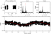 |
Fig. 1 Results of periodogram analysis of TOI-942. Top left panel: complete SuperWASP magnitudes time series vs. heliocentric Julian Day. Top middle panel: generalized Lomb-Scargle periodogram; the peak corresponding to the rotation period is indicated. Top right panel: CLEAN periodogram. Bottom panel: light curve phased with the rotation period. The solid line represents the sinusoidal fit. |
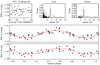 |
Fig. 2 Same as in Fig.1, but for the REM g′ filter. Also shown (bottom) is the r′ color curve phased with the rotation period. |
3.3.4 Frequency analysis of the HARPS-N data and stellar activity
We performed a frequency analysis of the HARPS-N RV measurements, and of the Ca II activity index (log  ) and CCF asymmetry indicator (BIS). The GLS periodogram (Zechmeister & Kürster 2009) of the HARPS-N RVs shows a significant peak at 3.373 days. By performing the bootstrap method (Murdoch et al. 1993; Hatzes 2016), which generates 10 000 artificial RV curves making random permutations from the real RV values, we estimated a FAP of 4%; although not highly significant due to the small number of RV data points, it clearly indicates the true rotation period. Similar values of periodicity are obtained for the log
  and BIS periodograms. Figure 4 displays the GLS for RVs, BIS, and log
  , together with the window function. It is clear that the stellar activity dominates the data. This is also revealed by the strong correlation between RVs and BIS (see Fig. 5), with Pearson and Spearman correlation coefficients equal to 0.92, and a significance of 2.38 × 10⁻⁷, evaluated through the IDL routine R_CORRELATE.
In order to further investigate the stellar activity, we produced the contour map of the residuals of the CCF11 versus radial velocity and rotational phase (Fig. 6). To obtain this map the single CCFs are subtracted from the mean CCF; positive deviations are shown in red and negative deviations are shown in blue. The RV variation due to stellar activity can be estimated from the associated perturbation of the intensity: ΔRV ≃ 2 × v sin i⋆ ×ΔI×f ≃ 470 ×f, where ΔI ~ 0.017 is the intensity range and f ≤ 1 the filling factor (Carleo et al. 2020b,a). The contours show that the activity of the star is dominated by one main active region, which remains quite coherent with the rotation period during the time span of our observations.
3.3.5 Rotation period
The various estimates of Prot derived above from photometric and spectroscopic time series agree with each other within 1σ; the small differences can be explained by differential rotation and evolution of active regions on the stellar surface. We adopt a weighted mean of the various determinations, 3.39 ± 0.01 days. The comparison with other clusters and groups of known age is discussed in Sect. 3.6.1.
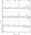 |
Fig. 4 From top to bottom: GLS of TOI-942 for HARPS-N RVs, BIS, and log |

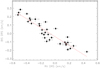 |
Fig. 5 Correlation between HARPS-N RVs and BIS of TOI-942. |
3.3.6 Projected rotational velocity
The projected rotational velocity v sin i⋆ was derived in two ways. In the first method we exploited the fast Fourier transform (FFT) method, as in Borsa et al. (2015). This method relies on the fact that it is possible to derive the v sin i⋆ from the first zero positions of the Fourier transform of the line profile (Dravins et al. 1990) when the rotational broadening is the dominant broadening component of the stellar line. The only prior information needed is the linear limb darkening coefficient; we adopted a value of 0.41, as found from the transit fit in Sect. 4. We applied the FFT method on the average mean line profile and obtained v sin i⋆ =13.9 ± 0.3 km s−1.
In the second mothod we used a preliminary calibration of the FWHM of the CCF built from other targets observed in the GAPS program (e.g., Borsa et al. 2015; Bonomo et al. 2017). We adopted the Doyle et al. (2014) relationship to take into account the contribution of the macroturbulence to the observed line width. We obtained in this way12 v sin i⋆=13.6 ± 0.7 km s−1. As the two determinations agree very well, we adopt the weighted average v sin i⋆=13.8 ± 0.5 km s−1.
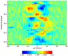 |
Fig. 6 Contour map of the CCF residuals of TOI-942 vs. radial velocity and rotational phase. The color bar indicates relative CCF amplitude with respect to the mean CCF. |
3.3.7 Coronal and chromospheric activity
The mean activity level on Ca II H and K lines, as measured with the procedure by Lovis et al. (2011) adapted to the HARPS-N spectra, results in log  = −4.17 ± 0.01, corresponding to 44 Myr using the Mamajek & Hillenbrand (2008) calibration. The star also appears very active when using the RAVE Ca IRT index (Žerjal et al. 2017), which corresponds to an age of 17 Myr with their calibration. Finally, the star was detected in the ROSAT all-sky survey (Voges et al. 2000), with the X-ray source identified as 1RXS J050636.4-201439. The resulting X-ray luminosity is high (logLX∕Lbol = −3.15), and is an indication of a very young star (formally 9 Myr using the Mamajek & Hillenbrand 2008 calibration).
3.4 Lithium
A very strong lithium 6708 Å doublet is seen in the spectra. We measured an equivalent width (EW) of 281 ± 5 mÅ, performing a Gaussian fit to the line profile using the IRAF task splot. The implications in terms of stellar age are discussed in Sect. 3.6.1.
3.5 Kinematics
The kinematics of TOI-942 are fully compatible with a young star, with U, V, and W space velocities (derived as in Johnson & Soderblom 1987) well inside the boundaries that determine the young disk population, as defined by Eggen (1996). The star is not a member of any known moving group derived by the application of BANYAN Σ online tool13 (Gagné et al. 2018a). This is not unexpected, considering the lack of members of known moving groups in the portion of the sky where the target is located (see, e.g., Fig. 5 in Gagné et al. 2018b). A search for comoving objects is presented in Appendix A. Two objects appear to have similar kinematics and isochrone age to TOI-942, and some indication of youth, and are probably comoving.
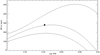 |
Fig. 7 Lithium EW vs. effective temperature for TOI-942 and sequences of ScoCen, IC 2602, and the Pleiades from Pecaut & Mamajek (2016). |
3.6 Stellar age, radius, and mass
In this section we present the analysis aimed at obtaining the stellar age, mass, radius, luminosity, and rotational velocity.
3.6.1 Stellar age
We compared the measurement of the age indicators for TOI-942 to those of members of open clusters or groups of known age. In this comparison we refer to the following: (i) the Pleiades open cluster and AB Dor moving group (MG) (age 125–149 Myr; Stauffer et al. 1998; Bell et al. 2015); (ii) the IC 2391 and IC 2602 open clusters, which have an age of 50 ± 5 and  Myr, respectively, from Li depletion boundary (Barrado y Navascués et al. 2004; Dobbie et al. 2010); and (iii) the Tuc-Hor, Columba, and Carina associations (age 42–45 Myr; Bell et al. 2015), and the β Pic MG (age 24–25 Myr; Bell et al. 2015; Messina et al. 2016).
The Li EW of TOI-942 (Fig. 7) is well above the median values of the Pleiades and AB Dor moving group (MG), although within the observed distributions (Desidera et al. 2015). The observed value is very close to the mean locus of Argus/IC 2391 (Desidera et al. 2011) and IC 2602 (Pecaut & Mamajek 2016) within the distribution of the members of nearby associations such as Tuc-Hor, Columba, and Carina (Desidera et al. 2015), and clearly below the locus of β Pic MG members (Messina et al. 2016). Therefore, the age of 40–150 Myr is inferred from the lithium EW, with a most probable age close to that of the young open clusters IC 2391 and IC 2602.
Figure 8 shows the comparison of the rotation period of TOI-942 with those of members of clusters and groups of known age. The rotation period of our target is clearly faster than those of Pleiades members falling on the I sequence (following the Barnes 2007 nomenclature), indicating a younger age, but slower than that of members of β Pic MG (Messina et al. 2017), confirming the older age found for lithium. Moreover, it is slightly faster than the members of the IC2391 open cluster and Argus association, and more compatible with the locus of the Tuc-Hor, Columba, and Carina associations (age 40–45 Myr).
The various indicators of magnetic activity are also consistent with an age of, at most, 150 Myr, although they are not able to precisely measure ages below 100 Myr. While the kinematics are fully compatible with a young age, the star is not associated with any known groups.
Finally, the position on the color-magnitude diagram (CMD) is slightly above the standard main sequence by Pecaut & Mamajek (2013)14, indicating a pre-main sequence status, and is close to the sequence of the single-star bona fide members of Tuc-Hor, Columba, and Carina from Gagné et al. (2018a) (Fig. 9). The position on the CMD of the seven possible comoving objects presented in Appendix A indicates a variety of ages. Two of them are close to the Tuc-Horsequence and are promising candidates for being coeval objects truly associated kinematically with TOI-942.
From the findings described above, the position on the CMD and the results of indirect methods such as lithium and rotation nicely agree on an age close to that of Tuc-Hor association and of IC2391 and IC2606 open clusters (45, 50, and 46 Myr, respectively; see above). Ages as young as β Pic MG (24–25 Myr) and as old as the Pleiades and AB Dor MG (125–149 Myr) are excluded by the data. We thus adopt an age of 50 Myr, with an age range of 30–80 Myr.
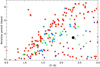 |
Fig. 8 Rotation period vs. V-K (corrected for reddening for the Pleiades) for TOI-942 (large black filled circle), and members of the Pleiades (red circles); IC 2391 (blue squares); Tuc-Hor, Columba and Carina associations (green triangles); and β Pic MG (purple upside-down triangles). References for rotation periods: Pleiades: Rebull et al. (2016); IC 2391: Messina et al. (2011), Desidera et al. (2011); Tuc-Hor, Columba, and Carina: Desidera et al. (in prep.), Messina et al. (2010, 2011); β Pic MG: Messina et al. (2017). |
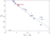 |
Fig. 9 Color-magnitude diagram of TOI-942 (red filled square) and of the possible comoving objects (blue filled squares; the number corresponds to the identification in Appendix A). Overplotted are the main sequence locus (continuous lines) from Pecaut & Mamajek (2013, updated version from the website), and the data of bona fide members from Gagné et al. (2018a) of the Tuc-Hor, Columba, and Carina associations (age 42–45 Myr, Bell et al. 2015), plotted as open circles. |
3.6.2 Stellar mass, radius, and luminosity
From the adopted Teff and the corresponding bolometric corrections from the Pecaut & Mamajek (2013) tables, we infer a stellar luminosity of  L⊙ and a stellar radius of
  R⊙. The stellar mass derived through the PARAM web interface (da Silva et al. 2006)15, isolating the age range allowed for the target, is 0.880 ± 0.031 M⊙.
As a sanity check, we derived the stellar parameters with the EXOFASTv2 tool (Eastman et al. 2019 Agol) by fitting the stellar SED and using the MIST stellar evolutionary tracks (Dotter 2016). For the SED we considered the WISE mid-IR W1, W2, and W3 magnitudes (Cutri & et al. 2013); the 2MASS near-IR J, H, and Ks magnitudes (Cutri et al. 2003); and the optical APASS Johnson B and V magnitudes, and Sloan g′, r′, and i′ magnitudes (Henden et al. 2016). We imposed a Gaussian prior on the Gaia parallax and uninformative priors on all the other parameters with upper bounds of 200 Myr and 0.050 on the stellar age and V-band extinction AV, respectively. We found R⋆ = 0.9286 ± 0.0087 R⊙, M⋆ = 0.912 ± 0.032 M⊙, L⋆ = 0.416 ± 0.006 L⊙, ρ⋆ = 1.605 ± 0.074 g cm−3, Teff = 4810 ± 23 K, ![$\textrm{[Fe/H]}=0.29^{+0.13}_{-0.16}$](/articles/aa/full_html/2021/01/aa39042-20/aa39042-20-eq16.png) dex, and a fairly precise age of 34 ± 6 Myr. The EXOFASTv2 analysis would thus indicate a possibly higher metallicity (though consistent with zero within 2σ), a slightly lower Teff, and younger age. Nonetheless, the stellar mass, radius, and age from EXOFASTv2 are fully consistent with the values that were independently derived above (i.e.,
dex, and a fairly precise age of 34 ± 6 Myr. The EXOFASTv2 analysis would thus indicate a possibly higher metallicity (though consistent with zero within 2σ), a slightly lower Teff, and younger age. Nonetheless, the stellar mass, radius, and age from EXOFASTv2 are fully consistent with the values that were independently derived above (i.e., 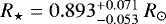 , M⋆ = 0.88 ± 0.031 M⊙, and age of
  Myr), which we adopt as the final stellar parameters for the more conservative uncertainties on the stellar radius and age.
In order to check this model-dependent result, we considered the dynamical masses derived for three objects of similar spectral type and comparable age, namely the components of the system HII2147 in the Pleiades open cluster (Torres et al. 2020) and AB Dor A in the AB Dor moving group (Azulay et al. 2017). Both AB Dor A and HII 2147B have G-band absolute magnitude slightly fainter than TOI-942 (5.75 and 5.8, respectively, versus 5.71), with a BP-RP color slightly bluer (1.10 and 1.08 versus 1.15, with the difference likely due to the slightly younger age of TOI-942). Their dynamical masses are 0.90 ± 0.08 M⊙ for AB Dor A and 0.879 ± 0.022 M⊙ for HII 2147B. The slightly brighter primary component of the HII2147 system (MG = 5.25, BP–RP = 0.97) has a dynamical mass of 0.978 ± 0.024 M⊙. We then conclude that the mass derived from models for TOI-942 is consistent with the available empirical dynamical masses of stars of comparable age. We then adopt the mass derived above, conservatively increasing the error bar to 0.04 M⊙ to take the systematic uncertainties of the models into account.
3.6.3 System inclination
Coupling the radius and the rotation period we obtain a rotational velocity of 13.3 km s−1, slightly smaller but very close to the observed v sin i⋆. The nominalparameters yield sin i⋆ slightly larger than unity. From the adopted error bars we obtain sin i⋆ = 1.04 . Considering only physical values we then have i > 70 deg. An alignment between the stellar equator and the orbits of the transiting planets is then very likely.
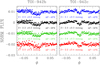 |
Fig. 10 Phased light curves for TOI-942 b (left panel) and TOI-942 c (right panel) obtained with different apertures marked with different colors. |
4 TESS photometric analysis and planet detection
A preliminary analysis of the TESS data allowed us to notice an additional signal in the light curve with a period of 10 days, associated with a second transiting planet.
In order to verify that TOI-942 b and TOI-942 c are genuine transiting candidates, we performed three different tests on the TESS light curve (see Sect. 3.1 of Nardiello et al. 2020 for a detailed description of the vetting tests). First, considering light curves obtained with different photometric methods, we verified that the depth of each single transit does not change. In Fig. 10 we compare the phased light curves centered for TOI-942 b (left panel) and TOI-942 c (right panel) obtained with different photometric apertures; for both the planets the shape and the depth of the transits obtained with different apertures are in agreement within 1σ. As a second test we checked whether the flux drops due to the transits and (X,Y)-positions obtained by PSF-fitting are correlated (Fig. 11); there is no clear correlation between the two quantities. The third test consists in the comparison between the depths of odd and even transits in order to exclude the possibility that the transits are due to a close eclipsing binary with different components. In panel a of Fig. 12 we indicate the position of the five transits of TOI-942 b (green) and two of TOI-942 c (blue). Panels b1 and b2 show the comparison between the average depths of odd and even transits for TOI-942 b and TOI-942 c, respectively: the odd and even transit depths are in agreement within 1σ. Finally, we computed the in-transit–out-of-transit difference centroid for the two transit signals in order to check whether the transits are due to a contaminant. As described in Nardiello et al. (2020), we calculated the centroid in a region of 10 × 10 TESS pixels (~210 × 210 arcsec2) centered on TOI-942 as follows. We selected the FFIs corresponding to the in-of-transits and out-of-transits points of the light curve and, for each transit, we calculated the stacked out-of-transit and in-of-transit image, and the difference between the two stacked images. For each transit, we calculated the photocenter on the out-of-transit–in-transit difference stacked image and its offset relative to the Gaia DR2 position of TOI-942. Finally, for each planet, we calculated the final in-transit–out-of-transit difference centroid as the mean of the offsets associated with the single transits. Panel c of Fig. 12 shows the results for the two exoplanets: in both cases, the in-transit–out-of-transit difference centroid to the position of TOI-942 is within the errors.
The transit fit was performed using the package PyORBIT16 (Malavolta et al. 2016, 2018), a package for modeling planetary transits and radial velocities while taking into account the effects of stellar activity and astrophysical contaminants. The transit modeling relies on the popular package batman (Kreidberg 2015).
We modeled the TESS light curve with a two-planet model (ecc2p), which includes the time of first transit Tc, the orbital period P, the eccentricity e and argument of periastron ω following the parameterization from Eastman et al. (2013) ( ,
, ), the limb darkening (LD) following Kipping (2013), the impact parameter b, and the scaled planetary radius RP∕R⋆. For each transit, the modulation induced by stellar activity is modeled by fitting a third-degree polynomial (to take into account the variability of the light curve over a few hours) on the out-of-transit part of the light curve around eachtransit event. A jitter term is included in order to take into account possible TESS systematics and short-term stellar activity noise. We implemented a Gaussian prior on the stellar density using the stellar mass and radius provided in Sect. 3. We made use of the parameterization, where the impact parameter b and the stellar density ρ⋆ are free parameters (e.g., Frustagli et al. 2020). Because no (bright) contaminants fall inside the photometric aperture adopted (red circle in panel c of Fig. 12), the dilution factor is negligible and is not included in the fit.
Modeling 7 transits and taking into account all the parameters described above, the number of free parameters of our model is 50. We ran the sampler for 100 000 steps, with 200 walkers, a burn-in cut of 20 000 steps, and a thinning factor of 100. In this way we obtained 147 200 independent samples. The posteriors confidence interval was computed by taking the 34.135th percentile from the median.
We also performed a transit fit with a circular model (circ2p). We computed the Bayesian information criterion (BIC) and the Akaike information criterion (AICc; corrected for small sample sizes), which is a second-order estimator of information loss, in order to assess the quality of our fits. We obtained that the circular fit is slightly preferred to the eccentric one (see Table 2), but it leads to a stellar density of 0.82 ± 0.09 ρ⊙. This value would require a full reshaping of the stellar parameters, inconsistent within the error bars. For this reason, we decided to adopt the eccentric fit to model our data, which leads to a stellar density consistent with the value obtained from spectroscopy (Sect. 3).
The TESS light curves, together with the resulting fits from the ecc2p model, are shown in Fig. 13. In addition, to visualize how the transit fit can change with varying transit parameters, we simulated several models for planet b for circular and eccentric orbits, and overplotted them on the nominal ecc2p model fit.
The fitted parameters, the adopted priors, and the parameter estimates obtained from the eccentric model are listed inTable 3. We found that the inner planet (TOI-942 b) has an orbital period of Pb = 4.3263 ± 0.0011 days and a radius Rb =  R⊕, while the outer planet (TOI-942 c) has an orbital period of Pc =
  days and a radius Rc =
  R⊕. We note that the periastron argument for both planets is ~268 deg; this is mainly due to a numerical bias, which leads to this configuration while minimizing the eccentricities and maximizing the transit duration. Another interesting aspect is the slightly eccentric orbit for TOI-942 b. While the transit data do not put significant constraints on the eccentricities, the transit duration, which is related to the stellar density, imposes a lower limit. Figure 14 shows the posterior distributions for the eccentricity of both planets. Because both are quite broad, we decided to adopt the peak values, which correspond to 0.285
 for TOI-942 b and 0.175
 for TOI-942 c. We also found that planet b andc have eccentricities ≤0.05 at 0.8% andat 8% cumulative percentages, respectively. We discuss the eccentricity issue further in Sect. 6.
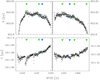 |
Fig. 11 Variation among the time of X and Y positions in pixel. Green triangles indicate the TOI-942 b transits, while blue triangle the TOI-942 c transits. |
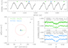 |
Fig. 12 Vetting procedure for TOI-942 b (green) and TOI-942 c (blue). Panel a: normalized light curve of TOI-942: green and blue arrows mark the position of the single transits of TOI-942 b and TOI-942 c, respectively. Panels b: comparison between the depths δ of the odd and even transits for the two exoplanets. Panel c: finding chart, centered on TOI-942 and based on the Gaia DR2 catalog: green and blue points represent the centroids computed analyzing the image obtained from the difference between theout- and in-of-transit stacked images; the red circle is the photometric aperture adopted in this work (see text and Nardiello et al. 2020 for details). |
Comparison between transit and RV models.
5 RV modeling
For the RV fit we employed the same package PyORBIT as for the light curve fit. Given the small sample size, and because the stellar activity is the predominant signal in our dataset, a proper planet detection from RVs was not possible. For the same reason, we did not perform a joint fit with the light curve. On the other hand, we could infer an upper limit on the mass of both planets.
We tested five different models to fit the HARPS-N RV data: (i) a circular two-planet with a Gaussian process (GP) model (circ2p+GP) to fit the stellar activity with a quasi-periodic kernel; (ii) an eccentric two-planet with a GP (ecc2p+GP); (iii) same as (ii), but with three planets (ecc3p+GP) to explore the possibility of an additional planetary companion; (iv) same as (iii), but adding a linear trend to check on a possible outer companion (ecc2p+GP+trend; see also Sect. 5.1); and (v) a GP-only model. The GP regression is performed through the package george (Ambikasaran et al. 2015); we employed the quasi-periodic kernel as defined by Grunblatt et al. (2015),
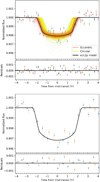 |
Fig. 13 Upper panel: TESS light curve around the transit with residuals of TOI-942 b. The black fit is the inferred ecc2p transit model, while the orange and yellow fits are respectively the eccentric and circular models obtained by randomly varying all the orbital parameters. Different dot colors indicate the five different transits for TOI-942 b. Bottom panel: TESS light curve around the two transits of TOI-942 c, with the ecc2p model overplotted. |
![\begin{equation*} h^2 \exp \biggl[-\frac{\sin^2{[\pi (t_i - t_j)/\theta]}}{2\omega^2} - \biggl(\frac{t_i - t_j}{\lambda}\biggr)^2\biggr], \end{equation*}](/articles/aa/full_html/2021/01/aa39042-20/aa39042-20-eq27.png) (2)
(2)
where h represents the amplitude of the correlations; θ is the rotation period of the star; ω is the length scale of the periodic component, which is related to the size evolution of the active regions; and λ represents the correlation decay timescale.
We ran the first four models performing a fit, which includes a Keplerian orbit for the planetary signal and independent jitter and offset terms. Using the orbital periods, the transit epochs obtained from the transit fit, and the eccentricity (in the case of eccentric models) as Gaussian priors, and the stellar parameters obtained in Sect. 3, we sampled the orbital period and the RV semi-amplitude in a linear space and followed the same parameterization as for the transit fit. We ran the sampler for 100 000 steps and 128 walkers. The burn-in cut and thinning factor are the same as reported in Sect. 4. We also computed the BIC and AICc criteria for the RV models. We report the results in Table 2; we find that the GP-only model is slightly preferred over the others. This is mainly due to the fact that the RVs cannot give a detection and are mostly dominated by the stellar activity. Moreover, the models with two planets are strongly preferred over the three planets case by both the BIC and the AICc, and in particular the circular model is favored over the eccentric one. These results are a consequence of the lack of a significant detection and the strong penalty given to models with a higher number of free parameters by the BIC and AICc criteria.
However, both circular and eccentric models return very similar parameter values. We found a jitter term related to the stellar activity of ~65 m s−1, and we assessed an upper limit to the RV semi-amplitudes, obtaining Kb < 7 m s−1 and Kc < 12 m s−1 corresponding to planetary masses of Mb < 16 M⊕ for planet b, and Mc < 37 M⊕ for planet c, at 1σ confidence level. These parameters, together with the GP model parameters, are listed in Table 3.
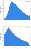 |
Fig. 14 Posterior distribution for the eccentricity of TOI-942 b (upper panel) and TOI-942 c (lower panel). The vertical red line indicates the maximum value of the distribution, while the dashed lines indicate the 16th and 84th percentiles. |
5.1 Contamination from possible stellar companions and line-of-sight objects
In order to evaluate the possibility of an astrophysical false positive caused by an eclipsing binary blended with TOI-942 in the TESS photometric aperture, we first considered the sources within 50′′ in Gaia DR2. As seen in Fig. 12, there is only one faint source, 2MASS J05063719-2014292 = TIC 146520534 at 23.4′′; however, it is ruled out as being responsible for the observed transit by the centroid test.
To estimate the chance for additional contaminants (either bound companions or field objects) we adopted the Gaia DR2 detection limits derived by Brandeker & Cataldi (2019). Considering targets with appropriate magnitude, the detection limits are of 2.25 mag at 1.0′′ and 9.0 mag at 4.0′′, corresponding to bound objects of mass 0.6 and <0.1 M⊙, at 150 and 600au, respectively.
We also used the TRILEGAL model of the Galaxy (Girardi et al. 2005) to simulate a population of stars along the line of sight: the number density of stars can be used to calculate the frequency of chance alignment given an aperture or radius of confusion. Using the Gaia contrast curve and the constraint from the transit depth of TOI-942 c, we obtained a maximum radius of 2.4 arcsec. The TRILEGAL simulation along the line of sight yields 821 bright enough stars per square degree. With the above-mentioned radius this yields an expected frequency of chance alignment of ~0.1%. Since the binary fraction is 33% (Raghavan et al. 2010) and the geometric transit probability for a 10.2-day orbit is ~1.5% (using the TOI-942 density and assuming a conservative maximum eclipse depth of 100%), which represents the fraction of binaries with the same period that would be eclipsing as viewed from Earth, we obtain a probability of 0.0005% that the signal is a background eclipsing binary (BEB). Repeating the same calculation for TOI-942 b, we obtained a slightly higher probability of 0.0007%. The probability of chance alignment with two different eclipsing binaries is the product of the two, which is extremely small (i.e., <10−10). So the likelihood is low that either signal is a BEB and very low that both are BEBs, given a total number of TESS targets of about 200 000. However, this analysis is rather conservative, since it does not take into account the transit shape, which would further eliminate BEB scenarios with incompatible radius ratios.
From the available systemic RVs in Table 1, small offsets are present between HARPS-N and Gaia DR2 and RAVE DR5. However, they are of marginal significance (less than 2σ in both cases, according to the nominal error bars). In addition, the HARPS-N RVs do not show significant trends within the timescale of our observations. An upper limit on the RV slope of 0.73 m s−1 d−1 (1σ confidence level) is obtained through a dedicated PyOrbit run including the presence of a linear trend. The CCF of our HARPS-N spectra also appears without signatures of additional components, although with the typical alterations of young spotted stars.
In order to assess the potential presence of additional non-transiting companions, we computed the minimum-mass detection thresholds of our HARPS-N RV time series. As previously done in Carleo et al. (2020b), we followed the Bayesian approach from Tuomi et al. (2014) to compute the detectability function and detection thresholds: we applied this technique on the RV residuals after correcting for the correlation with the BIS, and included in the model the signals of the two planets discussed in Sect. 5. Considering orbital periods between 0.5 and 200 d, we are sensitive to planets of minimum masses 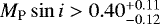 MJ, for 0.5 < P < 10 d, and
 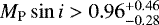 MJ for 10 < P < 200 d. For longer periods, due to the short baseline of our RV observations, our sensitivity drops and we are not sensitive even to the larger substellar companions.
Moreover, when considering the proper motion of the star from the most relevant astrometric catalogs such as Gaia DR2, Gaia DR1, Tycho2, PPMXL, SPM4.0, UCAC4, and UCAC5, no differences above 1.1σ are present, no astrometric excess noise is reported in Gaia DR2, and the re-normalized unit weight error (RUWE) is 1.07, well below the threshold of 1.4 indicating the need of additional parameters in the astrometric solution. All these results support the conclusion that there are no close companions that might represent a source of astrophysical false positive, or significantly dilute the observed transit depths, although the available detection limits do not rule out all the potential stellar companions to TOI-942.
TOI-942 parameters from the transit and RV fits.
5.2 False positive probability
We computed statistical false positive probabilities (FPPs) for TOI-942 b and TOI-942 c using the PYTHON package VESPA (Morton 2015). In brief, VESPA computes the likelihoods of astrophysical false-positive scenarios involving eclipsing binaries by comparing the observed transit shape with simulated eclipsing populations based on the TRILEGAL model of the Galaxy (Girardi et al. 2005). In particular, VESPA explores three different false positive scenarios: HEB (hierarchical eclipsing binary), EB (eclipsing binary), andBEB (background eclipsing binary – physically unassociated with target star). For planet b we find the FP probabilities PHEB = 0.06%, PEB = 3.13%, and PBEB ≪ 10−6. For planet c all the FPPs are <10−6.
However, because VESPA does not account for multiplicity, these FPPs are overestimated by at least an order of magnitude (Lissauer et al. 2012; Sinukoff et al. 2016; Livingston et al. 2018). Additionally, since the RVs put a constraint on the masses that rules out EBs, the planet probability would increase to over 99%. We thus consider both TOI-942 b and TOI-942 c to be statistically validated at the 99% confidence level.
6 Discussion
With both planets smaller than 5 R⊕ radii, and mass upper limits of 16 and 37 M⊕, this system appears to be very appealing for further analyses. We performed a study to investigate the evolution of the planetary atmospheres (Sect. 6.1), and we discussed the system architecture (Sect. 6.2) and the implications of the eccentric (Sect. 6.3) and circular (Sect. 6.4) orbit cases.
6.1 Atmospheric evolution simulations
We studied the atmospheric evolution of both planets evaluating the mass-loss percentage assuming circular orbits. The integrated stellar flux causing photoevaporation differs in the case of an eccentric orbit by  (i.e., by a factor of ~4% in the case of e = 0.285), implying that this approximation can be applied in our case. To estimate the atmospheric mass-loss rate we used the hydrodynamic-based approximation developed by Kubyshkina et al. (2018), including the evolution of the stellar extreme ultraviolet (XUV) luminosity and of the mass and radius of each planet, but neglecting the atmospheric gravitational contraction. In order to account for the X-ray stellar luminosity evolution we used the prescriptions given in Penz et al. (2008), whereas for the XUV radiation we used the relation given in Sanz-Forcada et al. (2011). We note that the above model for the XUV temporal evolution provides the evolution of the total X-ray luminosity distribution using a scaling law just for the mean value (Penz et al. 2008). For young stars the observed spread in X-ray luminosities is associated with the spread of stellar rotation rates (Pizzolato et al. 2003). The consequence of different rotation rates is that slow and fast rotators remain in the saturation regime for different time periods that go from about 10 Myr for slow rotators to about 300 Myr for fast rotators (Tu et al. 2015), implying very different levels of high-energy radiation to which planets are subjected. We account for the evolution of the radius following Johnstone et al. (2015). First, we estimate the radius of the rocky core, Rc, assuming that the density is equal to that of the Earth for both planets, and we obtain
  . Assuming a hydrogen dominated atmosphere, using Eq. (3) of Johnstone et al. (2015) and using the planetary radius given in Table 3, we estimate the initial atmospheric mass fraction fat = Mat∕Mpl; finally, at each time step we update fat and the planetary mass in response to the mass loss. Then using the new values for the mass and the atmospheric fraction we calculate the new radius.
Since the values for the mass in Table 3 are upper limits, and given the high uncertainty on the age of the star, for each planet a set of simulations was performed for three different values of the planetary mass, 1 × Mul,  ,
,  (where Mul = 16 M⊕ for TOI-942 b and Mul = 37M⊕ for TOI-942 c), and for stellar ages of 30, 50, and 80 Myr. For each simulation the initial X-ray luminosity is set at LX = 1030.07 erg s−1 (i.e., the initial mass-loss rate of the planets does not depend on the stellar age). The estimated initial atmospheric mass fractions for the three planetary masses in the case of TOI-942 b are 0.27, 0.19, 0.14, respectively; in the case of TOI-942 c they are 0.49, 0.5, 0.4, respectively.
For TOI-942 b the calculated current mass-loss rates are 1.31× 10¹³ g s−1, 2.05× 10¹⁴ g s−1, 1.03× 10¹⁵ g s−1, for the three masses 1 × Mul,  ,
,  , respectively. In the case of TOI-942 c, for the masses
  and
and  , we derived current mass-loss rates of 4.8 × 10¹² g s−1 and 1.2 × 10¹² g s−1, respectively, while for 1 × Mul the planet isstable against hydrodynamic evaporation and the mass-loss rate is negligible because the atmospheric losses are limited to Jeans escape.
Figure 15 shows the cumulative mass-loss percentage as a function of Δt = t − Tage (where t is the time and Tage the stellar age). In general and as expected, we found that in the case of high fat (high mass) the planet takes a longer time to lose its atmosphere; on the other hand, for a given mass, older stellar ages translate to shorter times needed to lose the envelope. This is basically due to the fact that the X-ray luminosity decays more slowly with time at older ages. The time taken to entirely lose the atmosphere goes from few Myr in the case of the lowest masses to Gyr in the case of highest masses. In particular, in the case of  TOI-942 b loses its atmosphere in less than 1 Myr, while in the case
  the planet’s atmosphere evaporates in about 2 Myr.
There are three scenarios for TOI-942 c: (i) in the case of  , it evaporates its atmosphere completely in approximately 200–300 Myr, depending on the stellar age; (ii) in the case of
  it loses its envelope only for the stellar age of 80 Myr in approximately 4.2 Gyr, while for the stellar ages of 30 and 50 Myr it only loses a fraction of its atmosphere in 5 Gyr; and (iii) in the case of 1 × Mul its atmosphere is hydrodynamically stable and the planet can only lose negligible amounts of its atmosphere through Jeans escape (hydrostatic evaporation).
When a planet loses its atmosphere entirely the final planetary radius value is given by the core radius value, which depends on the initial value of the planetary mass. On the other hand, when a planet loses only a fraction of its envelope, the final radius value depends on Eq. (3) of Johnstone et al. (2015). Generally, the radius distribution of close-in super Earths and sub-Neptunes follows a bi-modal distribution (for details see Fulton et al. 2017 or Modirrousta-Galian et al. 2020). As expected for this kind of planets, in the cases of  and
and  × Mul, and for all stellar ages, the radius of TOI-942 b, which initially lies on the right peak of the distribution, crosses the radius gap and ends its temporal evolution at the base of the left peak, which is likely populated by bare core planets.
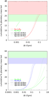 |
Fig. 15 Cumulative percentage of mass loss as a function of Δt = t − Tage. Red, green, and blue lines refer to planetary masses of 1 × Mul, |


6.2 System architecture
We briefly discuss here the planetary system around TOI-942 compared to other systems. It is interesting to understand whether young planetary systems have distinct features with respect to the mature ones that might shed light on their evolution. An analysis based on one individual system might be biased. A well-defined sample of young planetary systems is mandatory for a statistical evaluation.
Weiss et al. (2018) studied 909 planets in 355 multi-planet systems observed by Kepler, and found interesting and definite correlations among the characteristics of the planets. In particular, they found that planets in a multi-planet system present correlated masses or radii, and in 65% of cases the outer planets are larger than the inner planets. TOI-942 b and c, with respectively radii of 4.3 and 4.8 R⊕, follow the same trend. As discussed in Sect. 6.1, the planets of TOI-942, especially planet b, are expected to suffer from significant photoevaporation which changes their radii over time. Considering the evaporation model introduced in Sect. 6.1, the outer planet is expected to have a larger radius than the inner planet at all evolutionary stages. The larger relative shrinking of the radius of TOI-942 b would significantly change the ratio of the radii along the system evolution, but this should remain within the distribution of systems studied by Weiss et al. (2018), considering the difference in planet temperature.
We also examined the planetary separation in terms of mutual Hill radii (RH) in order to understand how far away from each other the two planets formed. We estimated the value of the planetary spacing as in Weiss et al. (2018), and we found that the TOI-942 planets have a separation of ~17 RH, in agreement with the Weiss et al. (2018) results which show that 93% of planet pairs are at least 10 mutual Hill radii apart17.
Moreover, we investigated the possible mean-motion resonances between the two planets. According to Fabrycky et al. (2014), most pairs of planets are not in mean-motion resonance. The period ratio between TOI-942 b and c is 2.349. This is close to the 7:3 ratio (2.333), corresponding to a minor peak in the Fabrycky et al. (2014) distribution.
6.3 Implications of eccentric orbits
In this section we discuss some implications that possible eccentric orbits for both planets can have on this system and our understanding of its history. TOI-942 b and c join the small group of Neptune-sized planets with orbital periods of a few days around late-type stars. These planets often present non-negligible orbital eccentricities, especially the subgroup with orbital periods shorter than ~10 days for which the mean value is ~0.15–0.20. A typical non-zero eccentricity for Neptunes in close orbits was also pointed out by Correia et al. (2020). The behavior of Neptune-radius planets in the period-eccentricity diagram is different with respect to giant planets, which show a clear increase in eccentricity at periods longer than 5 days, and to smaller planets (R < 3 R⊕), which typically have low eccentricity.
In order to understand the position of TOI-942 b and c in the same diagram, we reproduced the middle panel of Fig. 1 in Correia et al. (2020). We used Exo-MerCat (Alei et al. 2020), a Python software package that merges all the information from the four exoplanet catalogs, NASA Exoplanet Archive18 (Akeson et al. 2013), Exoplanet Orbit Database19 (Wright et al. 2011), Exoplanet Encyclopedia20 (Schneider et al. 2011), and Open Exoplanet Catalogue21 (Rein 2012), in order to have a unique, uniform, and standardized catalog. The Exo-MerCat catalog is publicly available as a VO resource and is updated weekly. We selected planets with orbital period 1 < Porb < 100 days, planetary radius 3 < RP < 9 R⊕, and eccentricity with uncertainties smaller than 0.1. Then we considered the eccentricities obtained for TOI-942 b and c from the transit fit (ecc2p) and added them to the sample (pink dots in Fig. 16). They follow the distribution within their uncertainties, although it is worth noting that our resulting eccentricities cannot be well constrained from our data, and while the circular model is preferred over the eccentric one, the latter leads to a consistent stellar density. Consequently, we cannot give any definitive conclusion on this aspect. An extensive RV survey would be needed to have a complete determination of the planet characteristics.
Assuming a modified tidal quality factor 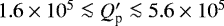 as suggested by the evolutionary scenario of the orbits of the main satellites of Uranus (Tittemore & Wisdom 1990; Ogilvie 2014), we estimate an e-folding decay timescale for the eccentricity22 of planet b ranging from 0.8 to 2.7 Gyr, while for planet c it ranges from 62 to 225 Gyr owing to the rapid decay of the tidal effects with the increase in the semi-major axis of the planetary orbit. A consequenceof tidal dissipation is the internal heating of planet b that provides a surface flux of about 575 W m−2 for
 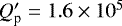 and scales in inverse proportion to the value of the tidal quality factor. It is much larger than in the case of Jupiter, which shows a flux of only 5.4 W m−2 (Guillot et al. 2004). In the case of planet c the tidally induced flux ranges from ~ 0.8 to ~ 3 W m−2 for the adopted range of
  , comparable with the value of the internal heat flux in Jupiter.
To gain insight into the implications of the eccentric model, we first verified the values of eccentricities for which the TOI-942 system could be stable through the Mean Exponential Growth factor of Nearby Orbits (MEGNO) (Cincotta & Simó 2000; Goździewski et al. 2008). MEGNO is closely related to the maximum Lyapunov exponent, providing an alternative determination of it. In the case of regular or quasi-periodic motion the MEGNO indicator is ≈2, while for chaotic motion it increases with time. To test the stability around the nominal orbit, we have regularly sampled the initial eccentricities of the two planets in the range 0.1–0.7 and computed the MEGNO for each orbit. In the numerical integrations spanning 50 Kyr, the initial semi-major axis and periastron argument of each planet are set to the nominal values, and the mutual inclination is equal to 0 since both planets transit the star.
To test the most difficult conditions for the dynamical stability of the system, we adopted the highest values for each planet mass: m1 = 16 M⊕ and m2 = 37 M⊕ (see Table 2). The results are shown as a stability map in Fig. 17. The stable area (blue region in the plot), where the values of MEGNO are close to 2, extends up to about 0.5 in eccentricity for both planets and the nominal solution is well within the stable region, suggesting that the high eccentricities derived from the system are not critical for its long-term stability.
We then investigated TOI-942’s dynamical history by means of its normalized angular momentum deficit (NAMD, Chambers 2001; Turrini et al. 2020), an architecture-agnostic measure of the dynamical excitation of a planetary system. The NAMD allows the dynamical excitation of planetary systems with diverse architectures to be compared, and provides insight into the differences in their dynamical histories (Turrini et al. 2020). We took advantage of this property to compare the dynamical excitation of TOI-942 with that of two template systems (Turrini et al. 2020): Trappist-1 (Gillon et al. 2017; Grimm et al. 2018)and the Solar System. Trappist-1’s dynamical history was shown to be characterized by stable and orderly evolution shaped by orbital resonances and tidal forces (Tamayo et al. 2017; Papaloizou et al. 2018). The Solar System, on the other hand, lies at the boundary between orderly and chaotic evolution, with signs of chaos and long-term instability in its current architecture and possible past phases of dynamical instability (e.g., Laskar & Petit 2017; Nesvorný 2018).
To compute the average NAMD value of TOI-942 taking into account the uncertainty in its physical and orbital parameters, we followed the Monte Carlo approach described by Laskar & Petit (2017) and Turrini et al. (2020). We performed 104 Monte Carlo extractions of the physical and orbital parameters of TOI-942’s planets and used them to compute the NAMD value of the resulting 104 simulated systems. For all parameters, we assumed standard deviations equal to half the confidence intervals of the respective quantities (Laskar & Petit 2017). Following Zinzi & Turrini (2017) and Turrini et al. (2020), we adopted as TOI-942’s reference plane the orbital plane of the largest planet, TOI-942 c, and converted the inclinations to relative inclinations with respect to this plane. As we possess only upper limits for the planetary masses we assumed that the two planets have similar densities (by analogy with Uranus and Neptune in the Solar System) and used their volumes in computing the NAMD (see also He et al. 2020). For the orbital eccentricities, we considered the posterior distributions for the planetary eccentricities shown in Fig. 14 truncated between zero and 0.5 to account for the results of the stability study with MEGNO.
Figure 18 shows the Monte Carlo lognormal distribution of TOI-942’s NAMD. The mean NAMD value is 3 × 10⁻² with the 3σ confidence interval extending from 4 × 10⁻³ to 0.3. Figure 18 also shows the NAMD values of Trappist-1 (2.4 ± 0.4 × 10⁻⁵) and of the Solar System (1.3 × 10⁻³). We refer readers to Turrini et al. (2020) for details on their computation. The NAMD values of Trappist-1 and the Solar System both fall well below TOI-942’s confidence interval, indicating that in the eccentric model, even if TOI-942 is currently dynamically stable, its dynamical history was more violent and chaotic than those of the other two systems. Using the full range of eccentricities and letting the planetary masses vary between Mul and 1∕3Mul (see Sect. 6.1) produces an analogous result, albeit with larger values for the mean NAMD and the upper boundary of the 3σ confidence interval. It is interesting to note that the period ratio close to 7:3 of TOI-942 b and c supports the picture depicted by TOI-942’s NAMD. The dynamical characterization of the 7:3 resonance in the asteroid belt (Gladman et al. 1997) shows how its timescale of ejection is on the order of a few tens of Myr (i.e., less than TOI-942’s age). If the two planets were originally trapped in a resonant condition (e.g., Xu & Lai 2017, and references therein), the eccentricity jump associated with their exit from it could be the violent dynamical event recorded by TOI-942’s NAMD value.
 |
Fig. 16 Distribution of eccentricities as a function of orbital period, as shown in Correia et al. (2020), for Neptune-sized planets. The eccentricities have uncertainties smaller than 0.1. TOI-942 b and c are overplotted in pink. |
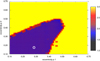 |
Fig. 17 MEGNO indicator computed for different initial values of the orbital eccentricity of the two planets. The color bar indicates the stability scale: the values of the MEGNO for the stable area is close to 2. Larger values of the MEGNO indicator (the yellow region) point to chaotic evolution. The star shows the nominal eccentricity values. |
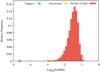 |
Fig. 18 NAMD lognormal distribution of the 104 Monte Carlo samples of TOI-942 computed varying the orbital and physical parameters of the two planets within their confidence intervals (see text for details). Also shown are the NAMD values of the Solar System (orange square) and Trappist-1 (blue square) for comparison. The horizontal positions of the Solar System and of Trappist-1 are arbitrary. |
6.4 Implications of circular orbits
If future investigations establish that TOI-942 b and c have circular orbits, this means that they could have migrated through a protoplanetary disk via a type I migration (e.g., Nelson 2018). The possibility that they formed via high-eccentricity migration is at variance with the very long circularization timescales, especially for planet c. Therefore, the possibility of explaining the eccentric orbits observed in similar systems as the residual of their formation through a high-eccentricity migration followed by sizeable evaporation of their atmospheres (Correia et al. 2020) does not appear applicable to our system in the case of circular orbits because the eccentricity of planet c did not change appreciably during its lifetime.
Testing the NAMD value of the planetary system in the circular case (i.e., accounting only for the dynamical excitation due to the relative inclination of the planets) returns a value only slightly higher than that of Trappist-1, suggesting an orderly evolution to the current architecture and further excluding the possibility of high-eccentricity migration.
7 Conclusions and future perspectives
In this paper we presented the validation of the Neptune-sized planet and the discovery of a second Neptune transiting the young star TOI-942 (TYC 5909-319-1, TIC 146520535), observed by TESS in Sector 5, with periods of 4 and 10 days, respectively. Thanks to TESS, REM, SuperWASP photometry, and HARPS-N spectroscopy we constrained most of the main stellar and planetary parameters. TOI-942 is a young and relatively active star with an age of  Myr and an activity index of log
  = −4.17 ± 0.01. TOI-942 b and c are Neptune-sized planets with a radius of 4.3 and 4.8 R⊕, and a mass upper limit of 16 and 37 M⊕, respectively. While the RV data do not present planet detections and are only used to infer an upper limit on the planetary masses because of the high stellar-activity jitter, the TESS light curves coupled with complementary spectroscopic, astrometric, and imaging datasets allow for system validation. Although the circular transit model is favored over the eccentric one, it leads to a stellar density value that is inconsistent with the stellar parameters obtained from the spectroscopy. This inconsistency disappears when the eccentricity is included in the model. In this case we found a slightly non-zero eccentricity for planet b. However, we note that the eccentricity distribution for each planet is the outcome of geometrical constraints (i.e., transit duration, impact parameter, and stellar density) since the poor sampling of the ingress or egress and the lack of a secondary eclipse do not allow for a precise determination of this parameter. Further RV observations are definitely important to better characterize the planetary masses and eccentricities, which will allow us to study the dynamical and evolution history of this system.
Our evaluations on planetary mass loss suggest that this system will be very interesting for future follow-up observations and atmospheric characterization. These kinds of systems with more than one planet play a very crucial role in understanding the physics behind the planetary formation process, and when all planets transit the star we have a great opportunity to obtain a comprehensive characterization of the system. We plan to keep monitoring this star in our GAPS program. Moreover, because TOI-942 is part of the CHEOPS sample, we will soon have very high-precision observations that will allow us to better refine the planetary radii, and to investigate the transit timing variations (TTVs) needed to explore the possibility of additional companions. The measurement of the Rossiter-McLaughlin effect would allow us to check the relative orientation of the planetary orbits and of the stellar spin. This is particularly relevant considering the young age and the possible dynamical history of the system.
Acknowledgements
This work has made use of data from the European Space Agency (ESA) mission Gaia (https://www.cosmos.esa.int/gaia), processed by the Gaia Data Processing and Analysis Consortium (DPAC, https://www.cosmos.esa.int/web/gaia/dpac/consortium). Funding for the DPAC has been provided by national institutions, in particular the institutions participating in the Gaia Multilateral Agreement. We acknowledge financial support from the ASI-INAF agreements n. 2018-16-HH.0 and 2018-22-HH.0, as well as the INAF Main Stream project ARIEL and the astrochemical link between circumstellar discs and planets (CUP: C54I19000700005). This paper includes data collected by the TESS mission. Funding for the TESS mission is provided by the NASA Explorer Program.
Appendix A Comoving objects
We looked for comoving objects around TOI-942 in order to have additional constraints on stellar age and to better characterize the environment of the planet host. We queried the Gaia DR2 catalog within 2 deg of the target for objects with a parallax difference smaller than 1 mas and proper motion difference smaller than 2 mas yr−1. Seven objects match these criteria (Table A.1). Star 7 has moderately blue colors from Gaia and Pan-STARRS (Chambers et al. 2016) and its position on the color-magnitude diagram is not compatible with a main sequence or pre-main sequence object; it lies slightly below the white dwarf sequence for the nominal parameters, but the astrometric parameters are highly uncertain. There is also a significantly brighter object at about 8″ (2MASS J05104749-1913475), that may bias photometric measurements.
The position on CMD of Fig. 9 shows that stars 3 and 4 (which actually form a wide binary with a projected separation of 13.3′′ ≃2100 au) are well above the standard main sequence and close to the empirical locus of Tuc-Hor, Columba, and Carina associations, suggesting that they are young. Their age appears fully compatible with our estimate for TOI-942. Stars 1, 2, 5, and 6 are instead close to the main sequence and could be older interlopers. The low absolute proper motion of TOI-942 might allow significant contamination by unrelated objects.
None of the targets has RV measurements from Gaia or other sources or signatures of being young, such as X-ray emission or UV excess due to chromospheric activity from GALEX. Only for stars 3 and 4 are there indications of photometricvariability: they are classified as RR Lyr candidates in Stringer et al. (2019). This classification is clearly not compatible with the position on CMD from Gaia, but can be the signature of short-period variability, considering the sparseness of their photometric measurements. We derived the photometric time series for all comoving candidates, with the exception of star 7 because of its faintness. Significant variability is detected for stars 3 and 4 (which are blended in the TESS data), with a possible periodicity of 0.47 d. This period would fit nicely the color- Prot sequence of the Pleiades (Rebull et al. 2016), especially if the observed period belongs to the brighter component (star 4). We conclude from the position of CMD and photometric variability that the wide binary system composed of 2MASS J05064475-1835567 and 2MASS J05064509-1836091 is likely coeval and comoving with TOI-942.
Comoving objects from Gaia.
Time series of TOI-942 from HARPS-N data.
References
- Akeson, R. L., Chen, X., Ciardi, D., et al. 2013, PASP, 125, 989 [NASA ADS] [CrossRef] [Google Scholar]
- Alei, E., Claudi, R., Bignamini, A., & Molinaro, M. 2020, Astron. Comput., 31, 100370 [CrossRef] [Google Scholar]
- Aleo, P. D., Sobotka, A. C., & Ramírez, I. 2017, ApJ, 846, 24 [CrossRef] [Google Scholar]
- Ambikasaran, S., Foreman-Mackey, D., Greengard, L., Hogg, D. W., & O’Neil, M. 2015, IEEE Trans. Pattern Anal. Mach. Intell., 38, 252 [NASA ADS] [CrossRef] [Google Scholar]
- Anglada-Escudé, G., & Butler, R. P. 2012, ApJS, 200, 15 [NASA ADS] [CrossRef] [Google Scholar]
- Azulay, R., Guirado, J. C., Marcaide, J. M., et al. 2017, A&A, 607, A10 [NASA ADS] [CrossRef] [EDP Sciences] [Google Scholar]
- Barnes, S. A. 2007, ApJ, 669, 1167 [NASA ADS] [CrossRef] [Google Scholar]
- Barrado y Navascués, D., Stauffer, J. R., & Jayawardhana, R. 2004, ApJ, 614, 386 [NASA ADS] [CrossRef] [Google Scholar]
- Bell, C. P. M., Mamajek, E. E., & Naylor, T. 2015, MNRAS, 454, 593 [NASA ADS] [CrossRef] [Google Scholar]
- Benatti, S., Nardiello, D., Malavolta, L., et al. 2019, A&A, 630, A81 [NASA ADS] [CrossRef] [EDP Sciences] [Google Scholar]
- Bonomo, A. S., Desidera, S., Benatti, S., et al. 2017, A&A, 602, A107 [NASA ADS] [CrossRef] [EDP Sciences] [Google Scholar]
- Borsa, F., Scandariato, G., Rainer, M., et al. 2015, A&A, 578, A64 [NASA ADS] [CrossRef] [EDP Sciences] [Google Scholar]
- Borucki, W. J., Koch, D., Basri, G., et al. 2010, Science, 327, 977 [NASA ADS] [CrossRef] [PubMed] [Google Scholar]
- Brandeker, A., & Cataldi, G. 2019, A&A, 621, A86 [NASA ADS] [CrossRef] [EDP Sciences] [Google Scholar]
- Butters, O. W., West, R. G., Anderson, D. R., et al. 2010, A&A, 520, L10 [NASA ADS] [CrossRef] [EDP Sciences] [Google Scholar]
- Carleo, I., Gandolfi, D., Barragán, O., et al. 2020a, AJ, 160, 114 [CrossRef] [Google Scholar]
- Carleo, I., Malavolta, L., Lanza, A. F., et al. 2020b, A&A, 638, A5 [CrossRef] [EDP Sciences] [Google Scholar]
- Casagrande, L., Ramírez, I., Meléndez, J., Bessell, M., & Asplund, M. 2010, A&A, 512, A54 [NASA ADS] [CrossRef] [EDP Sciences] [Google Scholar]
- Chambers, J. E. 2001, Icarus, 152, 205 [NASA ADS] [CrossRef] [Google Scholar]
- Chambers, K. C., Magnier, E. A., Metcalfe, N., et al. 2016, ArXiv e-prints [arXiv:1612.05560] [Google Scholar]
- Chincarini, G., Zerbi, F., Antonelli, A., et al. 2003, The Messenger, 113, 40 [NASA ADS] [Google Scholar]
- Cincotta, P. M., & Simó, C. 2000, A&AS, 147, 205 [NASA ADS] [CrossRef] [EDP Sciences] [Google Scholar]
- Correia, A. C. M., Bourrier, V., & Delisle, J. B. 2020, A&A, 635, A37 [CrossRef] [EDP Sciences] [Google Scholar]
- Cosentino, R., Lovis, C., Pepe, F., et al. 2012, Proc. SPIE Conf. Ser., 8446, 84461V [CrossRef] [Google Scholar]
- Crossfield, I. J. M., Waalkes, W., Newton, E. R., et al. 2019, ApJ, 883, L16 [CrossRef] [Google Scholar]
- Cutri, R. M., Skrutskie, M. F., van Dyk, S., et al. 2003, 2MASS All Sky Catalog of point sources [Google Scholar]
- Cutri, R. M. et al. 2013, VizieR Online Data Catalog: II/328 [Google Scholar]
- da Silva, L., Girardi, L., Pasquini, L., et al. 2006, A&A, 458, 609 [NASA ADS] [CrossRef] [EDP Sciences] [Google Scholar]
- David, T. J., Hillenbrand, L. A., Petigura, E. A., et al. 2016, Nature, 534, 658 [NASA ADS] [CrossRef] [PubMed] [Google Scholar]
- David, T. J., Petigura, E. A., Luger, R., et al. 2019, ApJ, 885, L12 [CrossRef] [Google Scholar]
- Desidera, S., Covino, E., Messina, S., et al. 2011, A&A, 529, A54 [NASA ADS] [CrossRef] [EDP Sciences] [Google Scholar]
- Desidera, S., Covino, E., Messina, S., et al. 2015, A&A, 573, A126 [NASA ADS] [CrossRef] [EDP Sciences] [Google Scholar]
- Dobbie, P. D., Lodieu, N., & Sharp, R. G. 2010, MNRAS, 409, 1002 [NASA ADS] [CrossRef] [Google Scholar]
- D’Orazi, V., & Randich, S. 2009, A&A, 501, 553 [NASA ADS] [CrossRef] [EDP Sciences] [Google Scholar]
- Dotter, A. 2016, ApJS, 222, 8 [NASA ADS] [CrossRef] [Google Scholar]
- Doyle, A. P., Davies, G. R., Smalley, B., Chaplin, W. J., & Elsworth, Y. 2014, MNRAS, 444, 3592 [Google Scholar]
- Dravins, D., Lindegren, L., & Torkelsson, U. 1990, A&A, 237, 137 [NASA ADS] [Google Scholar]
- Eastman, J., Gaudi, B. S., & Agol, E. 2013, PASP, 125, 83 [NASA ADS] [CrossRef] [Google Scholar]
- Eastman, J. D., Rodriguez, J. E., Agol, et al. 2019, PASP, submitted [arXiv:1907.09480] [Google Scholar]
- Eggen, O. J. 1996, AJ, 111, 1615 [NASA ADS] [CrossRef] [Google Scholar]
- Fabrycky, D. C., Lissauer, J. J., Ragozzine, D., et al. 2014, ApJ, 790, 146 [Google Scholar]
- Fossati, L., Erkaev, N. V., Lammer, H., et al. 2017, A&A, 598, A90 [NASA ADS] [CrossRef] [EDP Sciences] [Google Scholar]
- Frustagli, G., Poretti, E., Milbourne, T., et al. 2020, A&A, 633, A133 [CrossRef] [EDP Sciences] [Google Scholar]
- Fulton, B. J., Petigura, E. A., Howard, A. W., et al. 2017, AJ, 154, 109 [NASA ADS] [CrossRef] [Google Scholar]
- Gagné, J., Mamajek, E. E., Malo, L., et al. 2018a, ApJ, 856, 23 [NASA ADS] [CrossRef] [Google Scholar]
- Gagné, J., Roy-Loubier, O., Faherty, J. K., Doyon, R., & Malo, L. 2018b, ApJ, 860, 43 [NASA ADS] [CrossRef] [Google Scholar]
- Gaia Collaboration (Brown, A. G. A., et al.) 2018, A&A, 616, A1 [NASA ADS] [CrossRef] [EDP Sciences] [Google Scholar]
- Gandolfi, D., Fossati, L., Livingston, J. H., et al. 2019, ApJ, 876, L24 [Google Scholar]
- Gilbert, E. A., Barclay, T., Schlieder, J. E., et al. 2020, AJ, 160, 116 [CrossRef] [Google Scholar]
- Gillon, M., Triaud, A. H. M. J., Demory, B.-O., et al. 2017, Nature, 542, 456 [NASA ADS] [CrossRef] [PubMed] [Google Scholar]
- Girardi, L., Groenewegen, M. A. T., Hatziminaoglou, E., & da Costa, L. 2005, A&A, 436, 895 [NASA ADS] [CrossRef] [EDP Sciences] [Google Scholar]
- Gladman, B. J., Migliorini, F., Morbidelli, A., et al. 1997, Science, 277, 197 [NASA ADS] [CrossRef] [Google Scholar]
- Goździewski, K., Breiter, S., & Borczyk, W. 2008, MNRAS, 383, 989 [NASA ADS] [CrossRef] [Google Scholar]
- Grimm, S. L., Demory, B.-O., Gillon, M., et al. 2018, A&A, 613, A68 [NASA ADS] [CrossRef] [EDP Sciences] [Google Scholar]
- Grunblatt, S. K., Howard, A. W., & Haywood, R. D. 2015, ApJ, 808, 127 [NASA ADS] [CrossRef] [Google Scholar]
- Guillot, T., Stevenson, D. J., Hubbard, W. B., & Saumon, D. 2004, The interior of Jupiter, eds. F. Bagenal, T. E. Dowling, & W. B. McKinnon (Tucson: University of Arizona), 1, 35 [Google Scholar]
- Günther, M. N., Pozuelos, F. J., Dittmann, J. A., et al. 2019, Nat. Astron., 3, 1099 [Google Scholar]
- Hatzes, A. P. 2016, Astrophys. Space Sci. Lib., 428, 3 [CrossRef] [Google Scholar]
- He, M. Y., Ford, E. B., Ragozzine, D., & Carrera, D. 2020 AJ, 160, 276 [CrossRef] [Google Scholar]
- Henden, A. A., Levine, S., Terrell, D., & Welch, D. L. 2015, AAS Meeting Abstracts, 225, 336.16 [Google Scholar]
- Henden, A. A., Templeton, M., Terrell, D., et al. 2016, VizieR Online Data Catalog, 2336 [Google Scholar]
- Herbst, W., Bailer-Jones, C. A. L., Mundt, R., Meisenheimer, K., & Wackermann, R. 2002, A&A, 396, 513 [EDP Sciences] [Google Scholar]
- Huang, C. X., Burt, J., Vanderburg, A., et al. 2018, ApJ, 868, L39 [NASA ADS] [CrossRef] [Google Scholar]
- Hunter, A. A., Macgregor, A. B., Szabo, T. O., Wellington, C. A., & Bellgard, M. I. 2012, Source Code Biol. Med., 7, 1 [CrossRef] [Google Scholar]
- Johnson, D. R. H., & Soderblom, D. R. 1987, AJ, 93, 864 [NASA ADS] [CrossRef] [Google Scholar]
- Johnstone, C. P., Güdel, M., Stökl, A., et al. 2015, ApJ, 815, L12 [NASA ADS] [CrossRef] [Google Scholar]
- Kain, I., Mann, A., Newton, E., et al. 2019, AAS Meeting Abstracts, 233, 247.34 [Google Scholar]
- Kipping, D. M. 2013, MNRAS, 435, 2152 [Google Scholar]
- Kochanek, C. S., Shappee, B. J., Stanek, K. Z., et al. 2017, PASP, 129, 104502 [Google Scholar]
- Kreidberg, L. 2015, PASP, 127, 1161 [NASA ADS] [CrossRef] [Google Scholar]
- Kubyshkina, D., Fossati, L., Erkaev, N. V., et al. 2018, ApJ, 866, L18 [NASA ADS] [CrossRef] [Google Scholar]
- Kunder, A., Kordopatis, G., Steinmetz, M., et al. 2017, AJ, 153, 75 [Google Scholar]
- Lallement, R., Capitanio, L., Ruiz-Dern, L., et al. 2018, A&A, 616, A132 [NASA ADS] [CrossRef] [EDP Sciences] [Google Scholar]
- Lamm, M. H., Bailer-Jones, C. A. L., Mundt, R., Herbst, W., & Scholz, A. 2004, A&A, 417, 557 [NASA ADS] [CrossRef] [EDP Sciences] [Google Scholar]
- Laskar, J., & Petit, A. C. 2017, A&A, 605, A72 [NASA ADS] [CrossRef] [EDP Sciences] [Google Scholar]
- Leconte, J., Chabrier, G., Baraffe, I., & Levrard, B. 2010, A&A, 516, A64 [NASA ADS] [CrossRef] [EDP Sciences] [Google Scholar]
- Libralato, M., Bedin, L. R., Nardiello, D., & Piotto, G. 2016a, MNRAS, 456, 1137 [NASA ADS] [CrossRef] [Google Scholar]
- Libralato, M., Nardiello, D., Bedin, L. R., et al. 2016b, MNRAS, 463, 1780 [NASA ADS] [CrossRef] [Google Scholar]
- Lissauer, J. J., Marcy, G. W., Rowe, J. F., et al. 2012, ApJ, 750, 112 [NASA ADS] [CrossRef] [Google Scholar]
- Livingston, J. H., Endl, M., Dai, F., et al. 2018, AJ, 156, 78 [Google Scholar]
- Lovis, C., Dumusque, X., Santos, N. C., et al. 2011, ArXiv e-prints [arXiv:1107.5325] [Google Scholar]
- Malavolta, L., Nascimbeni, V., Piotto, G., et al. 2016, A&A, 588, A118 [NASA ADS] [CrossRef] [EDP Sciences] [Google Scholar]
- Malavolta, L., Mayo, A. W., Louden, T., et al. 2018, AJ, 155, 107 [NASA ADS] [CrossRef] [Google Scholar]
- Mamajek, E. E., & Hillenbrand, L. A. 2008, ApJ, 687, 1264 [NASA ADS] [CrossRef] [Google Scholar]
- Mann, A. W., Johnson, M. C., Vanderburg, A., et al. 2020, AJ, 160, 179 [CrossRef] [Google Scholar]
- Messina, S., Desidera, S., Turatto, M., Lanzafame, A. C., & Guinan, E. F. 2010, A&A, 520, A15 [NASA ADS] [CrossRef] [EDP Sciences] [Google Scholar]
- Messina, S., Desidera, S., Lanzafame, A. C., Turatto, M., & Guinan, E. F. 2011, A&A, 532, A10 [NASA ADS] [CrossRef] [EDP Sciences] [Google Scholar]
- Messina, S., Lanzafame, A. C., Feiden, G. A., et al. 2016, A&A, 596, A29 [NASA ADS] [CrossRef] [EDP Sciences] [Google Scholar]
- Messina, S., Lanzafame, A. C., Malo, L., et al. 2017, A&A, 607, A3 [NASA ADS] [CrossRef] [EDP Sciences] [Google Scholar]
- Minchev, I., Chiappini, C., & Martig, M. 2013, A&A, 558, A9 [NASA ADS] [CrossRef] [EDP Sciences] [Google Scholar]
- Modirrousta-Galian, D., Locci, D., & Micela, G. 2020, ApJ, 891, 158 [CrossRef] [Google Scholar]
- Morton, T. D. 2015, Astrophysics Source Code Library [record ascl:1503.011] [Google Scholar]
- Murdoch, K. A., Hearnshaw, J. B., & Clark, M. 1993, ApJ, 413, 349 [NASA ADS] [CrossRef] [Google Scholar]
- Nardiello, D., Bedin, L. R., Nascimbeni, V., et al. 2015, MNRAS, 447, 3536 [NASA ADS] [CrossRef] [Google Scholar]
- Nardiello, D., Libralato, M., Bedin, L. R., et al. 2016a, MNRAS, 455, 2337 [NASA ADS] [CrossRef] [Google Scholar]
- Nardiello, D., Libralato, M., Bedin, L. R., et al. 2016b, MNRAS, 463, 1831 [NASA ADS] [CrossRef] [Google Scholar]
- Nardiello, D., Borsato, L., Piotto, G., et al. 2019, MNRAS, 490, 3806 [CrossRef] [Google Scholar]
- Nardiello, D., Piotto, G., Deleuil, M., et al. 2020, MNRAS, 495, 4924 [CrossRef] [Google Scholar]
- Nelson, R. P. 2018, Handbook of Exoplanets (Berlin: Springer), 139 [Google Scholar]
- Nesvorný, D. 2018, ARA&A, 56, 137 [NASA ADS] [CrossRef] [Google Scholar]
- Newton, E. R., Mann, A. W., Tofflemire, B. M., et al. 2019, ApJ, 880, L17 [NASA ADS] [CrossRef] [Google Scholar]
- Nielsen, L. D., Gandolfi, D., Armstrong, D. J., et al. 2020, MNRAS, 492, 5399 [CrossRef] [Google Scholar]
- Nowak, G., Luque, R., Parviainen, H., et al. 2020, A&A, 642, A173 [NASA ADS] [CrossRef] [EDP Sciences] [Google Scholar]
- Ogilvie, G. I. 2014, ARA&A, 52, 171 [Google Scholar]
- Papaloizou, J. C. B., Szuszkiewicz, E., & Terquem, C. 2018, MNRAS, 476, 5032 [Google Scholar]
- Pecaut, M. J., & Mamajek, E. E. 2013, ApJS, 208, 9 [Google Scholar]
- Pecaut, M. J., & Mamajek, E. E. 2016, MNRAS, 461, 794 [Google Scholar]
- Penz, T., Micela, G., & Lammer, H. 2008, A&A, 477, 309 [NASA ADS] [CrossRef] [EDP Sciences] [Google Scholar]
- Perger, M., García-Piquer, A., Ribas, I., et al. 2017, A&A, 598, A26 [NASA ADS] [CrossRef] [EDP Sciences] [Google Scholar]
- Petigura, E. A., Sinukoff, E., Lopez, E. D., et al. 2017, AJ, 153, 142 [NASA ADS] [CrossRef] [Google Scholar]
- Pizzolato, N., Maggio, A., Micela, G., Sciortino, S., & Ventura, P. 2003, A&A, 397, 147 [NASA ADS] [CrossRef] [EDP Sciences] [Google Scholar]
- Plavchan, P., Barclay, T., Gagné, J., et al. 2020, Nature, 582, 497 [CrossRef] [Google Scholar]
- Quinn, S. N., Becker, J. C., Rodriguez, J. E., et al. 2019, AJ, 158, 177 [CrossRef] [Google Scholar]
- Raghavan, D., McAlister, H. A., Henry, T. J., et al. 2010, ApJS, 190, 1 [NASA ADS] [CrossRef] [EDP Sciences] [Google Scholar]
- Rebull, L. M., Stauffer, J. R., Bouvier, J., et al. 2016, AJ, 152, 113 [NASA ADS] [CrossRef] [Google Scholar]
- Rein, H. 2012, ArXiv e-prints [arXiv:1211.7121] [Google Scholar]
- Ricker, G. R., Winn, J. N., Vanderspek, R., et al. 2014, SPIE Conf. Ser., 9143, 914320 [Google Scholar]
- Rizzuto, A. C., Mann, A. W., Vanderburg, A., Kraus, A. L., & Covey, K. R. 2017, AJ, 154, 224 [NASA ADS] [CrossRef] [Google Scholar]
- Rizzuto, A. C., Newton, E. R., Mann, A. W., et al. 2020, AJ, 160, 33 [CrossRef] [Google Scholar]
- Roberts, D. H., Lehar, J., & Dreher, J. W. 1987, AJ, 93, 968 [Google Scholar]
- Sanz-Forcada, J., Micela, G., Ribas, I., et al. 2011, A&A, 532, A6 [NASA ADS] [CrossRef] [EDP Sciences] [Google Scholar]
- Schneider, J., Dedieu, C., Le Sidaner, P., Savalle, R., & Zolotukhin, I. 2011, A&A, 532, A79 [NASA ADS] [CrossRef] [EDP Sciences] [Google Scholar]
- Schuler, S. C., Plunkett, A. L., King, J. R., & Pinsonneault, M. H. 2010, PASP, 122, 766 [NASA ADS] [CrossRef] [Google Scholar]
- Sinukoff, E., Howard, A. W., Petigura, E. A., et al. 2016, ApJ, 827, 78 [NASA ADS] [CrossRef] [Google Scholar]
- Stassun, K. G., Oelkers, R. J., Pepper, J., et al. 2018, AJ, 156, 102 [NASA ADS] [CrossRef] [Google Scholar]
- Stauffer, J. R., Schultz, G., & Kirkpatrick, J. D. 1998, ApJ, 499, L199 [NASA ADS] [CrossRef] [Google Scholar]
- Stringer, K. M., Long, J. P., Macri, L. M., et al. 2019, AJ, 158, 16 [CrossRef] [Google Scholar]
- Takeda, Y., & Honda, S. 2020, AJ, 159, 174 [CrossRef] [Google Scholar]
- Tamayo, D., Rein, H., Petrovich, C., & Murray, N. 2017, ApJ, 840, L19 [NASA ADS] [CrossRef] [Google Scholar]
- Tittemore, W. C., & Wisdom, J. 1990, Icarus, 85, 394 [NASA ADS] [CrossRef] [Google Scholar]
- Torres, G., Melis, C., Kraus, A. L., et al. 2020, ApJ, 898, 2 [CrossRef] [Google Scholar]
- Tsantaki, M., Santos, N. C., Sousa, S. G., et al. 2019, MNRAS, 485, 2772 [NASA ADS] [CrossRef] [Google Scholar]
- Tu, L., Johnstone, C. P., Güdel, M., & Lammer, H. 2015, A&A, 577, L3 [NASA ADS] [CrossRef] [EDP Sciences] [Google Scholar]
- Tuomi, M., Jones, H. R. A., Barnes, J. R., Anglada-Escudé, G., & Jenkins, J. S. 2014, MNRAS, 441, 1545 [NASA ADS] [CrossRef] [Google Scholar]
- Turrini, D., Zinzi, A., & Belinchon, J. A. 2020, A&A, 636, A53 [CrossRef] [EDP Sciences] [Google Scholar]
- Voges, W., Aschenbach, B., Boller, T., et al. 2000, IAU Circ., 7432, 3 [NASA ADS] [Google Scholar]
- Weiss, L. M., Marcy, G. W., Petigura, E. A., et al. 2018, AJ, 155, 48 [Google Scholar]
- Wright, J. T., Fakhouri, O., Marcy, G. W., et al. 2011, PASP, 123, 412 [NASA ADS] [CrossRef] [Google Scholar]
- Xu, W., & Lai, D. 2017, MNRAS, 468, 3223 [CrossRef] [Google Scholar]
- Yee, S. W., Petigura, E. A., Fulton, B. J., et al. 2018, AJ, 155, 255 [NASA ADS] [CrossRef] [Google Scholar]
- Zechmeister, M., & Kürster, M. 2009, A&A, 496, 577 [NASA ADS] [CrossRef] [EDP Sciences] [Google Scholar]
- Žerjal, M., Zwitter, T., Matijevič, G., et al. 2017, ApJ, 835, 61 [NASA ADS] [CrossRef] [Google Scholar]
- Zhou, G., Quinn, S. N., Irwin, J., et al. 2021, AJ, 161, 2 [CrossRef] [Google Scholar]
- Zinzi, A., & Turrini, D. 2017, A&A, 605, L4 [NASA ADS] [CrossRef] [EDP Sciences] [Google Scholar]
From https://exoplanetarchive.ipac.caltech.edu/ on October 29, 2020.
Updated version available at http://www.pas.rochester.edu/ emamajek/EEM_dwarf_UBVIJHK_colors_Teff.txt, version 2019.3.22.
Updated version available at http://www.pas.rochester.edu/ emamajek/EEM_dwarf_UBVIJHK_colors_Teff.txt, version 2019.3.22.
Available at https://github.com/LucaMalavolta/PyORBIT
To be homogeneous with the analysis of Weiss et al. (2018) this estimate is derived for circular orbits and estimating the planetary masses from the empirical mass-radius relationships reported in Weiss et al. (2018).
All Tables
Main identifiers, equatorial coordinates, proper motion, parallax, magnitudes, and fundamental parameters of TOI-942.
All Figures
|
Fig. 1 Results of periodogram analysis of TOI-942. Top left panel: complete SuperWASP magnitudes time series vs. heliocentric Julian Day. Top middle panel: generalized Lomb-Scargle periodogram; the peak corresponding to the rotation period is indicated. Top right panel: CLEAN periodogram. Bottom panel: light curve phased with the rotation period. The solid line represents the sinusoidal fit. |
| In the text | |
|
Fig. 2 Same as in Fig.1, but for the REM g′ filter. Also shown (bottom) is the r′ color curve phased with the rotation period. |
| In the text | |
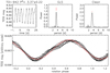 |
Fig. 3 Same as in Fig.1, but for the TESS time series. |
| In the text | |
|
Fig. 4 From top to bottom: GLS of TOI-942 for HARPS-N RVs, BIS, and log |
| In the text | |
|
Fig. 5 Correlation between HARPS-N RVs and BIS of TOI-942. |
| In the text | |
|
Fig. 6 Contour map of the CCF residuals of TOI-942 vs. radial velocity and rotational phase. The color bar indicates relative CCF amplitude with respect to the mean CCF. |
| In the text | |
|
Fig. 7 Lithium EW vs. effective temperature for TOI-942 and sequences of ScoCen, IC 2602, and the Pleiades from Pecaut & Mamajek (2016). |
| In the text | |
|
Fig. 8 Rotation period vs. V-K (corrected for reddening for the Pleiades) for TOI-942 (large black filled circle), and members of the Pleiades (red circles); IC 2391 (blue squares); Tuc-Hor, Columba and Carina associations (green triangles); and β Pic MG (purple upside-down triangles). References for rotation periods: Pleiades: Rebull et al. (2016); IC 2391: Messina et al. (2011), Desidera et al. (2011); Tuc-Hor, Columba, and Carina: Desidera et al. (in prep.), Messina et al. (2010, 2011); β Pic MG: Messina et al. (2017). |
| In the text | |
|
Fig. 9 Color-magnitude diagram of TOI-942 (red filled square) and of the possible comoving objects (blue filled squares; the number corresponds to the identification in Appendix A). Overplotted are the main sequence locus (continuous lines) from Pecaut & Mamajek (2013, updated version from the website), and the data of bona fide members from Gagné et al. (2018a) of the Tuc-Hor, Columba, and Carina associations (age 42–45 Myr, Bell et al. 2015), plotted as open circles. |
| In the text | |
|
Fig. 10 Phased light curves for TOI-942 b (left panel) and TOI-942 c (right panel) obtained with different apertures marked with different colors. |
| In the text | |
|
Fig. 11 Variation among the time of X and Y positions in pixel. Green triangles indicate the TOI-942 b transits, while blue triangle the TOI-942 c transits. |
| In the text | |
|
Fig. 12 Vetting procedure for TOI-942 b (green) and TOI-942 c (blue). Panel a: normalized light curve of TOI-942: green and blue arrows mark the position of the single transits of TOI-942 b and TOI-942 c, respectively. Panels b: comparison between the depths δ of the odd and even transits for the two exoplanets. Panel c: finding chart, centered on TOI-942 and based on the Gaia DR2 catalog: green and blue points represent the centroids computed analyzing the image obtained from the difference between theout- and in-of-transit stacked images; the red circle is the photometric aperture adopted in this work (see text and Nardiello et al. 2020 for details). |
| In the text | |
|
Fig. 13 Upper panel: TESS light curve around the transit with residuals of TOI-942 b. The black fit is the inferred ecc2p transit model, while the orange and yellow fits are respectively the eccentric and circular models obtained by randomly varying all the orbital parameters. Different dot colors indicate the five different transits for TOI-942 b. Bottom panel: TESS light curve around the two transits of TOI-942 c, with the ecc2p model overplotted. |
| In the text | |
|
Fig. 14 Posterior distribution for the eccentricity of TOI-942 b (upper panel) and TOI-942 c (lower panel). The vertical red line indicates the maximum value of the distribution, while the dashed lines indicate the 16th and 84th percentiles. |
| In the text | |
|
Fig. 15 Cumulative percentage of mass loss as a function of Δt = t − Tage. Red, green, and blue lines refer to planetary masses of 1 × Mul, |
| In the text | |
|
Fig. 16 Distribution of eccentricities as a function of orbital period, as shown in Correia et al. (2020), for Neptune-sized planets. The eccentricities have uncertainties smaller than 0.1. TOI-942 b and c are overplotted in pink. |
| In the text | |
|
Fig. 17 MEGNO indicator computed for different initial values of the orbital eccentricity of the two planets. The color bar indicates the stability scale: the values of the MEGNO for the stable area is close to 2. Larger values of the MEGNO indicator (the yellow region) point to chaotic evolution. The star shows the nominal eccentricity values. |
| In the text | |
|
Fig. 18 NAMD lognormal distribution of the 104 Monte Carlo samples of TOI-942 computed varying the orbital and physical parameters of the two planets within their confidence intervals (see text for details). Also shown are the NAMD values of the Solar System (orange square) and Trappist-1 (blue square) for comparison. The horizontal positions of the Solar System and of Trappist-1 are arbitrary. |
| In the text | |
Current usage metrics show cumulative count of Article Views (full-text article views including HTML views, PDF and ePub downloads, according to the available data) and Abstracts Views on Vision4Press platform.
Data correspond to usage on the plateform after 2015. The current usage metrics is available 48-96 hours after online publication and is updated daily on week days.
Initial download of the metrics may take a while.