| Issue |
A&A
Volume 628, August 2019
|
|
|---|---|---|
| Article Number | A89 | |
| Number of page(s) | 4 | |
| Section | Interstellar and circumstellar matter | |
| DOI | https://doi.org/10.1051/0004-6361/201935521 | |
| Published online | 12 August 2019 | |
Flaring water masers associated with W49N
1
Radio Astronomy Laboratory of Crimean Astrophysical Observatory,
Katsively
RT-22,
Crimea
e-mail: volvach@meta.ua
2
Institute of Applied Astronomy, Russian Academy of Sciences,
St. Petersburg, Russia
3
Astro Space Center, Lebedev Physical Institute, Russian Academy of Sciences,
Profsoyuznaya ul. 84/32,
Moscow
117997,
Russia
4
Hartebeesthoek Radio Astronomy Observatory,
PO Box 443,
Krugersdorp
1740,
South Africa
5
The University of Western Ontario,
1151 Richmond Street,
London,
ON N6A 3K7, Canada
6
Centre for Astronomy, Faculty of Physics, Astronomy and Informatics, Nicolaus Copernicus University,
Grudziadzka 5,
87-100
Torun,
Poland
7
Max-Planck-Institut für Radioastronomie,
Auf dem Hügel 69,
53121
Bonn,
Germany
8
National Astronomical Research Institute of Thailand,
260 Moo 4, T. Donkaew, A. Maerim,
Chiangmai
50180, Thailand
9
INAF, Istituto di Radioastronomia,
Via Gobetti 101,
40129
Bologna, Italy
10
Italian Alma Regional Centre, Istituto di Radioastronomia,
Via Gobetti 101,
40129
Bologna, Italy
11
INAF, Observatorio Astronomico di Cagliari,
Via della Scienza 5,
09047
Selargius (CA),
Italy
Received:
22
March
2019
Accepted:
11
July
2019
Aims. We present our monitoring observations and analysis of water masers associated with W49N taken in 2017 and 2018. A significant flare occurred during these observations.
Methods. We used ground-based radio telescopes in Simeiz (RT-22), Torun (RT-32), Medicina (RT-32), Effelsberg (RT-100) with broadband spectrometers. Observational data were collected and processed automatically.
Results. We report a powerful flare of the v = +6 km s−1 water maser feature; it increased in over ten months to S1.3 cm = 84 kJy in 2017 December, then decayed to the pre-flare quiescent value of S1.3 cm = 8.7 kJy in 2018 August. We infer that this flaring feature is unsaturated based on the relationship between line width and flux density.
Key words: masers / stars: formation / HII regions / radio lines: ISM
© ESO 2019
1 Introduction
The source W49N is one of the first in which the water maser emission at 22.235 GHz (616–523 transition) was detected (Knowles et al. 1969; Cheung et al. 1969). The total velocity extent of the water masers in W49N is ±300 km s−1. More than half of the maser features are located within a compact region of ~1 arcsec in diameter (Moran et al. 1973), which corresponds to ~0.05 pc given the distance to the source of 11 kpc (Zhang et al. 2013).
Most researchers prefer the mechanism of excitation of giant water masers in a wide range of speeds to shock waves created by the stellar wind coming from the central massive star of an early spectral class, and not related to accretion or radiation pressure (Strel’nitskii & Sunyaev 1972; Larson 1973; Hunter et al. 2018). Elitzur et al. (1989); Elitzur (1992) and Hollenbach et al. (2013) developed a picture in which the upper energy level of abundant H2O maser transition is pumped by collisions of the water molecules with H2 (Mac Low et al. 1994; Neufeld & Melnick 1991). Nevertheless, the sources of primary energy that cause the explosive process of maser radiation and the nature of flares in general remain unexplained (Gray et al. 2019).
W49N contains several ultra- and hyper-compact HII regions (Wynn-Williams 1971; De Pree et al. 2000), which coincide with the masering region. Becklin et al. (1973) detected an infrared (IR) source that is associated with W49N. The emission in the IR frequency regime is consistent with a black-body temperature of ~70 K.
The maser source W49N is associated with a radio-compact HII region with a radius smaller than 3.′′5 (Sato et al. 1967; Wynn-Williams 1971). The given angular value corresponds to 0.19 pc. At the distance of W49N, an early-type O5 star is required to produce a luminosity of L ~ 4 × 10⁵ L⊙ (Heckman & Sullivan 1976) and an excitation parameter u = 110 pc cm−2 to create a compact HII region. Thisenergetic stellar source is capable of ionising dense regions at a distance of 1017 −1018 cm from the central star.
Water maser flaring is a common occurrence in W49N. Sullivan (1973) detected a strong water maser flare in W49N, where its flux density rose to 80 kJy. Kramer et al. (2018) also reported a flare reaching 80 kJy in 2013–2014. Using very long baseline interferometry (VLBI), they found that the 2013–2014 flaring maser feature in W49N was near the centre of a north-south arc-like structure. Honma et al. (2004) similarly detected a strong flare in the same site in 2003 at v = −98 km s−1. The molecular water density can be significant in regions with maser activity. The abundance of H2 O relative to H2 is ~ 10−4, which is four to five orders of magnitude higher than the average ratio in the Galaxy (Harwit et al. 1998; Ceccarelli et al. 1998; Nisini et al. 1999; Maret et al. 2002). Water molecules, which evaporate at temperatures at about 130 K, become predominant in the protostellar medium, which might explain the flare peaks. Interestingly, Volvach et al. (2019a) reported two strong flares at the extreme velocity feature, v = − 81 km s−1; they suggested that this feature experienced significant flaring in 1976 (Little et al. 1977) and is unsaturated. We present the monitoring of water masers associated with W49N and the detection of a very powerful flaring event in 2017–2018. We also provide an analysis and interpretation of these data.
Parameters of the radio telescopes.
2 Observations
We observed at 22.235 GHz, which is the 616−523 water masertransition. Water maser observations were made with the 22 m Simeiz telescope (RT-22) using a spectropolarimetry radiometer and the parallel Fourier spectrum analyser (Volvach et al. 2010). The observation techniques at Torun Observatory, Poland, with the Effelsberg 100 m radio telescope in Germany, and with the Medicina1 32 m radio telescope in Italy were made in a similar way as those made at Simeiz (Table 1).
All observations were corrected in data reduction for atmospheric attenuation and telescope gain with respect to elevation. Each telescope was calibrated using known calibrator continuum sources (using cross-scan mode), for instance, 3C286 and NGC7027 (Kraus et al. 2003; Perley & Butler 2013). A current version of the program “Field system” was employed by the RT-22 at Simeiz; this allowed management of all standard and non-standard devices by a single server (Vandenberg 1995). Non-standard devices and software included a broadband radiometer, a wideband spectrometer, an RDR recorder, and the RT-22 radio telescope control system.
The Medicina RT-32 was operated in its standard configuration as described by Melis et al. (2015), allowing us to observe left- and right-hand circular polarizations simultaneously in four bands of 2048 channels each and with progressively higher resolution in zoom mode. Observations were completed in position-switching mode, the offset position was 0. °5 to the east of the source. Left- and right-hand polarization spectra were processed separately and then averaged to obtain a total of 12 min ON-source integration. Pointing checks were performed typically every 1–2 h using quasars. The observations were corrected for atmospheric opacity, which was determined from fitting a model atmosphere to skydip observations. Skydips were performed afew times per observing session.
Monitoring observations of the water masers associated with W49N began in 2017 September and were conducted in parallel with the observations of water masers associated with G025.65 + 1.05, where another powerful flare was recorded. The observation cadence was every one to two days (Fig. 1).
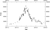 |
Fig. 1 Time-series plot of the flux density of the ~+6 km s−1 water maserfeature associated with W49N. Circles denote the RT-22 Simeiz data, diamonds represent the RT-32 Torun data, squares represent the RT-100 Effelsberg data, and stars represent the RT-32 Medicina data. |
3 Results
The time series of the v = +6 km s−1 velocity channel for our W49N water maser observations during 2017 and 2018 is presented in Fig. 1. The velocity channel clearly experienced a significant flaring event. The event increased from ~8.7 to ~84 kJy in 2017 December, in about ten months. It returned to a quiescent state in a similar time span. On closer inspection, there appears to be episodic flaring as it increased to its maximum flux density. During the decay phase the event went through a secondary and much weaker flare.
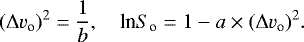
We present water maser spectra from each telescope in Fig. 2. The RT-100 Effelsberg spectrum was taken on 2017 August 14 during the onset of the flare, and the other two were taken at or near the flare maximum. It is clear from the RT-100 spectra that this is a complex maser source, and the singular and relatively narrow +6 km s−1 maser feature is evident. Evidence of flaring in other channels is visible at the 10 kJy level in Fig. 2b. Figure 3 shows the Medicina RT-32 spectrum, which was taken after this feature returned to its pre-flare state on 2018 July 31. A single component with a width ≅ 0.67 km s−1 at vLSR ≈ +6 km s−1 accounts for a significant portion (more than 95%) of the total flux density at the peak of the flare.
Complex spectra, such as the water masers associated with W49N presented here, are typified by significant line feature overlap. However, Fig. 2b shows that the feature at +6 km s−1 is narrow, the average line width Δv0 = 1.04 km s−1, and it is notaffected by line overlap during the flares. We are therefore confident that during the flaring phase a fit with Gaussian profiles, in particular to the flaring feature, will yield representative results. In Fig. 4 we plot the inverse of the square of the line width versus the natural logarithm of the flux density for the +6 km s−1 water maserfeature. The errors of the data are represented by the velocity resolution during observations (from 0.05 to 0.1 km s−1). There appears to be a linear relationship. The best-fitting line is described by
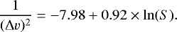 (1)
(1)
4 Discussion
Significant water maser flaring activity, brighter than 10 kJy, has been reported previously by Hirota et al. (2014) for Orion KL, by Volvach et al. (2019b) for G25.65+1.05, and by Volvach et al. (2019a) for W49N. The authors reported a relationship between line width and flux density thatis similar to what we observed here. We compare the results in Table 2, where Δv0 is the initial line half-width, S0 is the initial flux density, a and b are the coefficients from the fitted linear equation 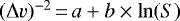 , the gain, and finally, the residual mean square (σ).
The experimental dependence of the line width versus flux density, for example, that presented in Fig. 4 and the results listed in Table 2, is derived from Goldreich & Kwan (1974):
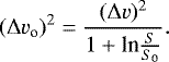 (2)
(2)
Transforming Eq. (2) into Eq. (1), we obtain the expressions for Δv0 and S0 :
 (3)
(3)
The flares share the proportionate relationship between  and lnS, which implies that each flaring maser feature is unsaturated (Goldreich et al. 1973). The results are not obviousy correlated in any other way. One result of interest is that S0 > S1.3 cm (continuum); it is not clear why. Perhaps the continuum emission rose markedly prior to the onset of the water maser flare. Alternatively, a foreground maser may be amplifying the emission from a background maser along the same line of sight.
The resulting values of Δvo for each analysed flare are about 1 km s−1. This corresponds to T ≈ 240 K for H2 molecules. This temperature is insufficient to provide effective pumping of the masers when we consider that the vaporization temperature of water molecules is T ≈ 130 K (Strel’nitskii 1982). We show in Fig. 4 that the line width becomes more narrow as the maser strength increases, which means that the maser feature is unsaturated. The light curve (Fig. 1) is strikingly similar, in terms of temporal behaviour and duration, to the time series of the water maser flare in Orion KL that was reported by Shimoikura et al. (2005). These authors also concluded that the flaring maser feature was in an unsaturated state.
Water maser emission in the velocity channel v = +6 km s−1 flared and grew exponentially. Goldreich et al. (1973) noted that the exponential increase in flux density is associated with a similar change in the optical thickness of the maser source. The optical thickness does not exceed unity, therefore radiation from the entire volume of the maser spot occurs. Rapid rise in flux density in individual flares can be associated with shock pumping from passing narrow plasma fronts, and rapid decays may be due to the so-called drying up of water (Heckman & Sullivan 1976).
These significant water maser flaring events might be a consequence of a sharp rise in temperature (up to 103 K), density (up to 1011 cm−3), and ionization levels (ne /nH = 10−5). This may have been initiated by a collision–collision (CC) maser pumping mechanism (Strel’nitskii 1982). The primary energy release may be associated with a partial ejection of a stellar shell or rapid strengthening of the stellar wind from the central star caused by gravitational pressure at periastron of multiple star systems (Volvach et al. 2019b). Rapid changes in physical conditions in maser spots may be the result of powerful shock waves generated by cataclysmic occurrences in a massive central star. The preferred ejection direction depends on the orientation of the orbit of the multiple system. This may explain the fact that in different maser sources, high velocity maser features dominate. They are either extreme blue- or red-shifted.
Pikelner & Strel’nitskiy (1976) and Norman & Silk (1979) both considered the effects of stellar winds on masers. If the gas is heated by a shock wave, the energy dissipates firstly into heavier particles, for example, the abundant hydrogen atoms and water molecules. Electrons remain cooler throughout the passage of the shock wave. Secondly, these hydrogen atoms and water molecules excite the rotational water levels, while electrons provide a cooling mechanism. This means that water masers may be activated by shock waves from stellar winds. The pump frequency (Γ) exceeds the stimulated emission rate (R) (Goldreich et al. 1973). In this case the maser increased exponentially with the pumping rate. Figure 1 shows that the maser flux density increases exponentially during the flare. This may also indicate that the large increase in the maser intensity during flaring (by factors of hundreds) can be explained by an unsaturated maser.
It can be argued that the flare depicted in Fig. 1 is comprised of several (possibly five or six) flares of shorter duration. Likewise, this can be argued for the flares described in Volvach et al. (2019a). The time between these two flares was about one to two months, and the duration of each flare was about one year. Interferometric observations by Moran et al. (1973) and Knowles et al. (1974) showed that water masers are found in maser clusters. We estimate that the size of possible maser clusters where successive flaring may be occurring is about 1015 cm across when the propagation velocity of the disturbance is assumed to be ~200 km s−1. The three star-forming regions (Orion KL, G25.65+1.05, and W49N) where significant flaring activity (Speak > 20 kJy) has occurred have similar characteristics in terms of their time series, flare durations, and other details, including those listed in Table 2. They are found in clusters in which flaring is occurring. Certainly all were unsaturated. To successfully advance our understanding of the structure and dynamics of maser regions, simultaneous monitoring observations on single radio telescopes and the global interferometer are desirable.
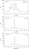 |
Fig. 2 Light curve of +6 km s−1 of W49N taken in 2017. Panel a: Effelsberg spectrum (August 14). Panel b: Simeiz spectrum (December 24). Panel c: Torun spectrum (December 26). |
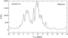 |
Fig. 3 H2O maser emission spectra of W49N taken in 2018: Medicina (July 31). |
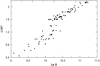 |
Fig. 4 Relationship between the flux density and line width of the water maser feature at +6 km s−1 associated with W49N during the 2017–2018 flare. |
Comparison between the W49N and G25.65+1.05 water masers during each flare event.
5 Conclusions
We reportedthe detection of the largest water maser flare associated with W49N between 2017 September and 2018 December. The water maser feature at ~+6 km s−1 reached a peak flux density ~84 kJy. This flaring was confirmed by contemporaneous observations in Poland, Germany, and Italy. We find that like the other flaring sources, this feature is unsaturated during the flaring phase. We propose that the processes that occur during these massive flares in the sources Orion KL, G25.65+1.05, and W49N are similar. More observations, both interferometric mapping and maser monitoring, are needed to better understand these exciting fast-flaring maser phenomena.
Acknowledgements
The authors acknowledge support from the National Science Centre, Poland, through grant 2016/21/B/ST9/01455. This work was partially supported by Program 12 of the Russian Academy of Sciences. Partly based on observationswith the Effelsberg 100 m telescope of the Max-Planck-Institut für Radioastronomie in Effelsberg. We wish to thank the Maser Monitoring Organisation (M2O), a group of loosely organised radio telescopes that coordinates and cooperates for observations, for its prompt response for our request for confirmatory observations and increased monitoring of water masers associated with W49N.
References
- Becklin, E. E., Neugebauer, G., & Wynn-Williams, C. G. 1973, ApJ, 13, L147 [Google Scholar]
- Ceccarelli, C., Caux, E., White, G. J., et al. 1998, A&A, 331, 372 [NASA ADS] [Google Scholar]
- Cheung, A. C., Rank, D. M., Townes, C. H., Thornton, D. D., & Welch, W. J. 1969, Nature, 221, 626 [NASA ADS] [CrossRef] [Google Scholar]
- De Pree, C. G., Wilner, D. J., Goss, W. M., Welch, W. J., & McGrath, E. 2000, ApJ, 540, 1, 308 [NASA ADS] [CrossRef] [Google Scholar]
- Elitzur, M., Hollenbach, D. J., & McKee, C. F. 1989, ApJ, 346, 983 [NASA ADS] [CrossRef] [Google Scholar]
- Elitzur, M., Hollenbach, D. J., & McKee, C. F. 1992, ApJ, 394, 221 [NASA ADS] [CrossRef] [Google Scholar]
- Goldreich, P., & Kwan, J. 1974, ApJ, 191, 93 [NASA ADS] [CrossRef] [Google Scholar]
- Goldreich, P., Keeley, D. A., & Kwan, J. J. 1973, ApJ, 179, 111 [NASA ADS] [CrossRef] [Google Scholar]
- Gray, M. D., Baggott, J., Westlake, J., & Etoka, S. 2019, MNRAS, 486, 4216 [NASA ADS] [CrossRef] [Google Scholar]
- Harwit, M., Neufeld, D. A., Melnik, G. J., & Kaufman, M. J. 1998, ApJ, 497, 105 [NASA ADS] [CrossRef] [Google Scholar]
- Heckman, T. M., & Sullivan, W. T. 1976, ApJ, 17, L105 [Google Scholar]
- Hirota, T., Kim, M. K., & Honma, M. 2014, ApJ, 797, L35 [NASA ADS] [CrossRef] [Google Scholar]
- Hunter, T. R., Brogan, C. L., & Bartkiewicz, A. 2018, ASP Conf. Ser., 517, 321 [NASA ADS] [Google Scholar]
- Hollenbach, D. J., Elitzur, M., & McKee, C. F. 2013, ApJ, 773, 25 [Google Scholar]
- Honma, M., Choi, Y. K., Bushimata, T., et al. 2004, PASJ, 56, L15 [NASA ADS] [CrossRef] [Google Scholar]
- Knowles, S. H., Mayer, C. H., Cheung, A. C., Rank, D. M., & Townes, C. H. 1969, Science, 163, 1055 [NASA ADS] [CrossRef] [PubMed] [Google Scholar]
- Knowles, S. H., Johnston, K. J., Moran, J. M., et al. 1974, AJ, 79, 925 [NASA ADS] [CrossRef] [Google Scholar]
- Kramer, B. H., Menten, K. M., & Kraus, A. 2018, IAU Symp., 336, 279 [NASA ADS] [Google Scholar]
- Kraus, A., Krichbaum, T. P., & Wegner, R. 2003, A&A, 401, 161 [NASA ADS] [CrossRef] [EDP Sciences] [Google Scholar]
- Larson, R. B. 1973, ARA&A, 1973, 219 [NASA ADS] [CrossRef] [Google Scholar]
- Little, L. T., White, G. J., & Riley, P. W. 1977, MNRAS, 180, 639 [NASA ADS] [CrossRef] [Google Scholar]
- Mac Low, M.-M., Elitzur, M., Stone, J. M., & Konigl, A. 1994, ApJ, 427, 914 [NASA ADS] [CrossRef] [Google Scholar]
- Maret, S., Caccarelli, C., Caux, E., Tielens, A. G. G. M., & Castels, A. 2002, A&A, 395, 573 [NASA ADS] [CrossRef] [EDP Sciences] [Google Scholar]
- Melis, A., Migoni, C., Comoretto, G., et al. 2015, SRT internal report 52, http://www.oa-cagliari.inaf.it/area.php?page_id=10 [Google Scholar]
- Moran, J. M., Papadopoulos, G. D., & Burke, B. F., 1973, ApJ, 185, 535 [NASA ADS] [CrossRef] [Google Scholar]
- Neufeld, D. A., & Melnick, G. J. 1991, ApJ, 368, 215 [NASA ADS] [CrossRef] [Google Scholar]
- Nisini, B., Benedettini, M., & Giannini, T. 1999, A&A, 350, 529 [NASA ADS] [Google Scholar]
- Norman, C., & Silk, J. 1979, ApJ, 228, 197 [NASA ADS] [CrossRef] [Google Scholar]
- Perley, R. A., & Butler, B. J. 2013, ApJS, 204, 19 [NASA ADS] [CrossRef] [Google Scholar]
- Pikelner, S. B., & Strel’nitskiy, V. S. 1976, Astrophys. Space Sci., 39, L19 [CrossRef] [Google Scholar]
- Sato, F., Akabane, F., & Kerr, F. J. 1967, Aust. J. Phys., 20, 197 [NASA ADS] [CrossRef] [Google Scholar]
- Shimoikura, T., Kobayashi, H., & Omodaka, T. 2005, ApJ, 634, 459 [NASA ADS] [CrossRef] [Google Scholar]
- Strel’nitskii, V. S. 1980, Astron. Lett., 6, 354 [Google Scholar]
- Strel’nitskii, V. S. 1982, Astron. Lett., 8, 165 [Google Scholar]
- Strel’nitskii, V. S., & Sunyaev, R. A. 1972, AZh, 49, 704 [NASA ADS] [Google Scholar]
- Sullivan, W. T. 1973, ApJS, 25, 393 [NASA ADS] [CrossRef] [Google Scholar]
- Vandenberg, N. R. 1995, NASA/Goddard Space Flight Center [Google Scholar]
- Volvach, L. N., Volvach, A. E., & Strepka, I. D. 2010, 20th International Conference Microwave & Telecommunication Technology, Sevastopol, 1189 [Google Scholar]
- Volvach, L. N., Volvach, A. E., & Larionov, M. G. 2019a, MNRAS, 487, L77 [NASA ADS] [CrossRef] [Google Scholar]
- Volvach, L. N., Volvach, A. E., & Larionov, M. G. 2019b, MNRAS, 482, L90 [NASA ADS] [CrossRef] [Google Scholar]
- Wynn-Williams, C. G. 1971, MNRAS, 151, 397 [NASA ADS] [Google Scholar]
- Zhang, B., Reid, M. J., & Menten, K. M. 2013, ApJ, 775, 13 [Google Scholar]
All Tables
Comparison between the W49N and G25.65+1.05 water masers during each flare event.
All Figures
|
Fig. 1 Time-series plot of the flux density of the ~+6 km s−1 water maserfeature associated with W49N. Circles denote the RT-22 Simeiz data, diamonds represent the RT-32 Torun data, squares represent the RT-100 Effelsberg data, and stars represent the RT-32 Medicina data. |
| In the text | |
|
Fig. 2 Light curve of +6 km s−1 of W49N taken in 2017. Panel a: Effelsberg spectrum (August 14). Panel b: Simeiz spectrum (December 24). Panel c: Torun spectrum (December 26). |
| In the text | |
|
Fig. 3 H2O maser emission spectra of W49N taken in 2018: Medicina (July 31). |
| In the text | |
|
Fig. 4 Relationship between the flux density and line width of the water maser feature at +6 km s−1 associated with W49N during the 2017–2018 flare. |
| In the text | |
Current usage metrics show cumulative count of Article Views (full-text article views including HTML views, PDF and ePub downloads, according to the available data) and Abstracts Views on Vision4Press platform.
Data correspond to usage on the plateform after 2015. The current usage metrics is available 48-96 hours after online publication and is updated daily on week days.
Initial download of the metrics may take a while.