| Issue |
A&A
Volume 625, May 2019
|
|
|---|---|---|
| Article Number | A32 | |
| Number of page(s) | 46 | |
| Section | Extragalactic astronomy | |
| DOI | https://doi.org/10.1051/0004-6361/201834675 | |
| Published online | 07 May 2019 | |
Study of gravitational fields and globular cluster systems of early-type galaxies
1
Astronomical Institute, Czech Academy of Sciences, Boční II 1401/1a, 141 00 Prague, Czech Republic
e-mail: bilek@asu.cas.cz
2
Faculty of Mathematics and Physics, Charles University in Prague, Ke Karlovu 3, 121 16 Prague, Czech Republic
3
Astronomical Observatory, Volgina 7, 11060 Belgrade, Serbia
4
Lund Observatory, Sövegatan 27, Box 43, 221 00 Lund, Sweden
Received:
17
November
2018
Accepted:
25
February
2019
Context. Gravitational fields at the outskirts of early-type galaxies (ETGs) are difficult to constrain observationally. It thus remains poorly explored how well the ΛCDM and MOND hypotheses agree with ETGs.
Aims. The dearth of studies on this topic motivated us to gather a large sample of ETGs and examine homogeneously which dark matter halos they occupy, whether the halos follow the theoretically predicted stellar-to-halo mass relation (SHMR) and the halo mass-concentration relation (HMCR), whether ETGs obey MOND and the radial acceleration relation (RAR) observed for late-type galaxies (LTGs), and finally whether ΛCDM or MOND perform better in ETGs.
Methods. We employed Jeans analysis of radial velocities of globular clusters (GCs). We analysed nearly all ETGs having more than about 100 archival GC radial velocity measurements available. The GC systems of our 17 ETGs extend mostly over ten effective radii. A ΛCDM simulation of GC formation helped us to interpret the results.
Results. Successful ΛCDM fits are found for all galaxies, but compared to the theoretical HMCR and SHMR, the best-fit halos usually have concentrations that are too low and stellar masses that are too high for their masses. This might be because of tidal stripping of the halos or because ETGs and LTGs occupy different halos. Most galaxies can be fitted by the MOND models successfully as well, but for some of the galaxies, especially those in centers of galaxy clusters, the observed GC velocity dispersions are too high. This might be a manifestation of the additional dark matter that MOND requires in galaxy clusters. Additionally, we find many signs that the GC systems were perturbed by galaxy interactions. Formal statistical criteria prefer the best-fit ΛCDM models over the MOND models, but this might be due to the higher flexibility of the ΛCDM models. The MOND approach can predict the GC velocity dispersion profiles better.
Key words: gravitation / galaxies: elliptical and lenticular, cD / galaxies: kinematics and dynamics / galaxies: interactions / galaxies: halos / galaxies: clusters: general
© ESO 2019
1. Introduction
The missing mass problem has not been solved decisively yet. The two most discussed solutions are the standard cosmological ΛCDM model (e.g., Mo et al. 2010) and the MOND paradigm of modified dynamics (Milgrom 1983, 2015; Famaey & McGaugh 2012). In this paper we aim to test their predictions in early-type galaxies (ETGs).
Assuming the ΛCDM paradigm, galaxies are surrounded by dark matter halos whose density can be described well by the Navarro-Frenk-White (NFW) profile (Navarro et al. 1996) according to dark-matter-only cosmological simulations. These halos are expected to meet the stellar-to-halo mass relation (SHMR) between the stellar mass of the galaxy and the mass of its dark halo (e.g., Behroozi et al. 2013). This relation is supposed to exist because the transport of baryons inside or outside the halo depends on the mass of the halo; the more massive the halo is, the more it accretes satellites and intergalactic gas. On the other side, the processes expelling the baryons from the halos such as active galactic nuclei outflows, supernova explosions, and stellar winds are less effective if the baryons reside in a deeper potential well. This relation can be recovered, for example, by the abundance matching technique based on comparing the halo mass function deduced from cosmological simulations to the observed galaxy stellar mass function while assuming that the most massive galaxies lie within the most massive halos; i.e., the recovered SHMR is a combination of results from observations and simulations. We must remember that the recovered SHMR is not necessarily the SHMR that ΛCDM would predict in a perfect simulation, which would include, for example, all baryonic processes correctly. In the current hydrodynamical cosmological simulations the parameters regulating the baryonic processes have to be tuned so that the galaxy stellar mass function matches the observations (Genel et al. 2014; Crain et al. 2015; Pillepich et al. 2018). The simulations that are not explicitly tuned to reproduce the stellar mass function do not do so properly (Khandai et al. 2015; Kaviraj et al. 2017).
Another correlation that the dark matter halos are expected to follow is that between the halo mass and its concentration referred to as the halo mass-concentration relation (HMCR). The concentration, c, of a NFW halo is the virial radius of the halo divided by its scale radius. The HMCR is a result deduced from ΛCDM cosmological simulations.
The MOND paradigm consists in a change of the laws of inertia or gravity in weak gravitational fields. In other words, according to MOND we encounter the missing mass problem mainly because the laws of general relativity are not valid for weak gravitational fields just as the laws of Newtonian dynamics are not valid for strong gravitational fields. In MOND, test particles move approximately obeying the equation
where a is the actual acceleration of the particle and aN is the acceleration predicted by the Newtonian dynamics on the basis of the distribution of the observable matter. The interpolation function μ switches gradually between the Newtonian regime (μ(x) ≈ 1) for strong gravitational fields (x ≫ 1) and the deep-MOND regime (μ(x) ≈ x) for weak gravitational fields (x ≪ 1). The transition between these regimes occurs at the critical acceleration of a0 ≈ 1.2 × 10⁻¹⁰ m s−2. The expected deviations from Eq. (1) depend on the particular MOND theory, mass distribution, and orbital shape (Bekenstein & Milgrom 1984; Milgrom 1994, 2010; Ciotti et al. 2006; Brada & Milgrom 1995).
For every galaxy, we can construct an empirical radial acceleration relation (RAR) between the observed acceleration, a, and aN (McGaugh et al. 2016). Observations show that most late-type galaxies (LTGs) follow the RAR predicted by MOND in Eq. (1) (e.g., Begeman et al. 1991; Sanders 1996; de Blok & McGaugh 1998; Milgrom & Sanders 2007; Gentile et al. 2011; Angus et al. 2012a; McGaugh et al. 2016; Lelli et al. 2017; Milgrom 2017; Li et al. 2018). The other attempts to solve the missing mass problem have to explain this empirical fact as well. The attempts to do so in the ΛCDM framework employ other empirical relations whose validity is not an inevitable result of hydrodynamic simulations such as the SHMR (see, e.g., Di Cintio & Lelli 2016; Navarro et al. 2017). The form of RAR and the validity of MOND are much less explored in ETGs than in LTGs.
This is because investigating the gravitational fields of ETGs is more complicated than in LTGs. In the ΛCDM context, a specific problem is the fact that most of the visible objects in galaxies extend toward galactocentric radii substantially smaller than the characteristic radii of their dark halos and therefore the parameters of the profiles are difficult to constrain, especially given that the mass of stars in a galaxy is also uncertain. When testing MOND, we encounter a similar problem. We need tracers of gravitational potential at large radii where MOND predicts measurable deviations from the Newtonian gravity without dark matter, i.e., where the gravitational accelerations are much below a0. Otherwise we can just test whether the data are consistent with no deviation. When investigating the gravitational fields of the ETGs, we usually rely on the Jeans analysis of the radial velocities of some kinematic tracers whose motion are fully governed by the gravitational field, such as stars, planetary nebulae, globular clusters (GCs), and satellites. However the shape of the trajectories is unknown and this introduces uncertainties in the measurement; some constraints can be inferred from the higher order moments of the tracer velocity distribution (see Sect. 3). Neighboring galaxies can disturb the tracers from virial equilibrium. It is also possible to use stellar shells to investigate the gravitational fields of ETGs up to large radii (Ebrová et al. 2012; Bílek et al. 2015, 2016) but faint shells are difficult to detect. Another method relies on the hydrostatic equilibrium between the pressure of the hot interstellar gas and the gravitational field. The obstacle in this approach is that the equilibrium might not be perfect, for example, because of a recent activity of the galactic nucleus. In addition, the gravitational field cannot usually be investigated up to the radii where the gravitational acceleration is expected to be substantially weaker than a0. Milgrom (2012) tested MOND successfully down to very low accelerations in two ETGs with unusually high amounts of hot gas. Some ETGs also contain rotating H I disks. Weijmans et al. (2008) used these to verify MOND in one ETG down to the acceleration comparable to a0 and Lelli et al. (2017) extended this results to a sample of 16 ETGs. Investigations of gravitational fields using gravitational lensing have the advantage of not relying on the uncertain assumptions such as the hydrostatic equilibrium or the shape of the orbits of kinematic tracers. The strong gravitational lensing allows the determination of the dynamical mass enclosed below a certain galactocentric radius. If a galaxy follows MOND, we can never probe the regions where the accelerations are substantially lower than a0 using this method (Milgrom 2012). Tian & Ko (2017) used strong lensing to verify MOND down to the acceleration comparable with a0 in a few tens of ETGs. Weak gravitational lensing can be used to probe the gravitational field up to large galactocentric distances but at the price of galaxy stacking. If some of the galaxies have an unusual gravitational field and for example they do not agree with MOND, then we will not learn about their existence. Milgrom (2013) verified the consistency of MOND with weak galaxy-galaxy lensing up to very large radii in red galaxies (presumably ETGs) and blue galaxies (presumably LTGs).
In summary, the tests of MOND in ETGs were generally positive. Only the works based on the Jeans modeling of the radial velocities of various tracers in the ETGs gave controversial results (Tiret et al. 2007; Angus 2008; Richtler et al. 2008, 2011; Samurović & Ćirković 2008, 2009; Tortora et al. 2014; Samurović et al. 2014; Samurović 2014, 2016a,b, 2017; Dabringhausen et al. 2016; Samurović & Vudragović 2019). Recent examples include the work by Janz et al. (2016), who concluded that the spatially resolved kinematics of their 14 fast rotator ETGs is in tension with MOND. On the contrary, Rong et al. (2018) found that the spatially resolved kinematics of the fast rotator ETGs in the MaNGA survey are consistent with MOND but they identified an inconsistency with the slow rotators. Finally, Lelli et al. (2017) claimed that the RAR of the LTGs works in all galaxies universally, including the slow rotators.
While Jeans analysis has its down sides, it still enables, as one of few methods, investigating the gravitational fields of individual ETGs beyond a few effective radii of the starlight of the galaxy if the GCs are used as the kinematic tracers. Observing the radial velocities of GCs is a demanding task requiring a lot of observing time at large telescopes. In the present work, we collect a sample of 17 ETGs that includes nearly all galaxies for which over 100 GC radial velocities have been measured. The GC systems often extend over 10 effective radii of the galaxy. Together with the real galaxies, we study in the same way the GCs of a galaxy formed in a hydrodynamical ΛCDM simulation. Our main motivation is to test the above predictions of ΛCDM and MOND, i.e., whether the GC kinematics can be modeled well given the assumed gravitational law and observational constraints, and whether the SHMR, HMCR, and RAR hold true in our galaxies. If we find that these predictions are not met, we will attempt to find an explanation, which is usually an influence of the environment.
This paper is organized as follows. We present our sample of real and simulated galaxies in Sect. 2 where we also describe the methods used to obtain the stellar mass-to-light ratios from galaxy colors. In Sect. 3, we derive the observational characteristics of the studied GC systems. In Sect. 4 we describe how we computed the theoretical velocity-dispersion profile for a given gravitational field of the galaxy. Our maximum a posteriori method to model the kinematics of the GCs is presented in Sect. 5 and the results to which it led in Sect. 5.2. We deal with the predictions of the velocity dispersion profiles of the GC systems by the ΛCDM and MOND paradigms based on independent estimates of the free parameters in Sect. 6. We also investigated in Sect. 7 the RARs using the GC systems. All results are discussed in Sect. 8; specifically, we discuss the possible reason of deviations from the ΛCDM predictions in Sect. 8.1 and from the MOND predictions in Sect. 8.2. We summarize our work and build the final picture following from it in Sect. 9.
Throughout the paper, we denote the decadic logarithm by log and the natural logarithm by ln. For consistency with Behroozi et al. (2013) whose results we are building on, we adopt a flat cosmology with the parameters H0 = 70 km s−1, Ωm = 0.27, Ωb = 0.046, σ8 = 0.8 and ns = 0.96. This is consistent with the WMAP5 (Komatsu et al. 2009) and the WMAP7+BAO+H0 (Komatsu et al. 2011) cosmologies.
2. Galaxy sample and used data
2.1. Real galaxies
In this paper we analyze the following 17 nearby ETGs: NGC 821, NGC 1023, NGC 1399, NGC 1400, NGC 1407, NGC 2768, NGC 3115, NGC 3377, NGC 4278, NGC 4365, NGC 4472, NGC 4486, NGC 4494, NGC 4526, NGC 4649, NGC 5128, and NGC 5846. We study their dynamics based on their observed GCs, which we do not split into red and blue subpopulations; rather we work with the whole sample of objects. The velocity errors for the objects are typically below 20 km s−1 and they rarely exceed 30 km s−1. Since one of the main tasks of this study is to analyze the problem of the missing mass it was important that the available data extend out to several effective radii (Re) for each ETG for which large deviations from Newtonian dynamics without dark matter are expected. Thus, the galactocentric distance of the outermost point expressed in the units of Re varies from 4.5 (for NGC 3115) to 30.2 (for NGC 1399). The galaxies were chosen so as to have at least 100 confirmed GCs, where NGC 821 and NGC 1400 are the exception, with 68 objects in each galaxy and the largest number of GCs are available in the case of NGC 1399 for which 790 objects were used. Such numbers of tracers are not sufficient to establish the exact anisotropy in a given bin accurately because as shown in Merritt (1997) at least several hundred tracers per bin are necessary for this purpose. Therefore, our estimates of the s3 and s4 parameters below are to be understood merely as an indicator of anisotropies. All type of ETGs are included in the sample, from round (for example, NGC 5846) to flattened (for example, NGC 3377) ellipticals to lenticulars (for example, NGC 3115). The selected galaxies belong to various environments: there are 2 field galaxies (NGC 821 and NGC 3115), 6 cluster galaxies, and 9 galaxies that belong to groups. We also note that our sample features both fast and slow rotators, and the fast rotators are more numerous (12 fast versus 5 slow rotators). In all our calculations we took into account the systemic rotation, which varies from approximately zero (such as NGC 821, NGC 1399, and NGC 5846) to 140 km s−1 (NGC 4526 and NGC 4649). Their colors vary from those that resemble their spiral counterparts (NGC 3377) to red (NGC 1407). The observational data for our galaxies are taken from several publicly available databases and the details are as follows. The main part of our sample, namely the galaxies NGC 821, NGC 1023, NGC 1400, NGC 1407, NGC 2768, NGC 3115, NGC 3377, NGC 4278, NGC 4365, NGC 4486 (=M 87), NGC 4494 NGC 4526, and NGC 5846 come from the SLUGGS (SAGES Legacy Unifying Globulars and Galaxies Survey, where SAGES is the Study of the Astrophysics of Globular Clusters in Extragalactic Systems) sample1 (Forbes et al. 2017). The data for the remaining four galaxies are available in the following papers: Schuberth et al. (2010) for NGC 1399, Côté et al. (2003) for NGC 4472 (=M 49), Lee et al. (2008) for NGC 4649 (=M 60), and Woodley et al. (2010) for NGC 5128 (=Centaurus A). The basic observational data for the galaxies in the sample is available in Table 1 and the information related to GCs is available in Table 2.
Galaxy sample.
Properties of globular cluster systems.
2.2. Artificial galaxies
Together with the real galaxies, we analyzed the GC system of the galaxy from the simulation by Renaud et al. (2017). We used these data to generate artificial observations, which helped us to check the correctness of our methods and interpret the results. This simulation is a zoom-in on a Milky Way-like galaxy in the ΛCDM framework with Planck cosmology (see also Li et al. 2017; Kim et al. 2018). The spatial resolution of this simulation was ∼200 pc and the dark matter particles had a mass of 2.1 × 10⁶ M⊙. The simulation includes injection of energy and momentum, and chemical enrichment (in Fe and O) from SN type II and Ia, stellar winds, and radiative pressure. It also implements a metallicity-dependent cooling and heating from UV background.
The radial profile of the cumulated baryonic mass of the simulated galaxy has a distinct plateau between around 10–100 kpc where it maintains the value of 4.8 × 10¹⁰ M⊙, which we identify as the baryonic mass of the galaxy. The galaxy has the r200 radius below which the average dark matter density is 200 times the Universe critical density of 184 kpc. We fitted the cumulated-mass profile of the dark matter particles with a NFW profile (Eq. (12)) up to the radius of r200. We obtained log(ρs [M⊙ kpc−3]) = 6.72 and log(rs [kpc]) = 1.29. Such a NFW halo has the M200 mass of 7 × 10¹¹ M⊙ and a concentration of c = 9.4.
We created three artificial galaxies from this single simulated galaxy by making its projection along the Cartesian axes of the simulation. We then treated the projections as separate galaxies, which we labeled as R17x, R17y, and R17z (or collectively as R17x,y,z). The actual distance of these three galaxies was assumed to be 21 kpc, which is a typical distance to our real galaxies. We however pretended in the following that the observed distance to these galaxies is 19 kpc in order to simulate the observational errors. The difference is the typical 1σ error given by Tonry et al. (2001) for their measurements at this distance. The artificial galaxies were all assumed to have an actual M/L = 4.7, a typical M/L predicted by the SPS models for our real galaxies. We generated images of the artificial galaxies with the resolution of 0.25″ pixel−1 and the field of view (FOV) of 12′×12′. These images were then fitted by a Sérsic profile using Galfit (Peng et al. 2002). The resulting structural parameters are presented in Table 1. The SPS M/Ls for the R17x,y,z galaxies were copied from NGC 3115 because it is a fast rotator with a similar stellar mass. We identified the GC particles in the same way as Renaud et al. (2017), i.e., as the stellar particles formed before 10 Gyr. We randomly chose 200 GCs so that their maximum galactocentric radius was 15 Re to mimic the data for the real galaxies. We then created for the RG17x,y,z, galaxies artificial catalogs of the apparent GC positions and radial velocities. These data were subsequently treated in the same way as the data for the real galaxies. Finally, we obtained the systemic rotation velocity of the GC systems using the standard method described, for example, in Richtler et al. (2004).
The RARs of the R17x,y,z galaxies are plotted in the panels f of Figs. C.18–C.20 by the dotted yellow lines. These were obtained in the following way. We calculated a nearly true Newtonian gravitational acceleration in each of these galaxies from the stellar distribution obtained by fitting its artificial image and from the correct values (without the intentionally added error) of the galaxy distance and M/L. In order to obtain the dynamical acceleration of the galaxy, we added to the baryonic acceleration the force from the above-described NFW halo. We can see that the galaxies follow well the RAR of the LTGs depicted by the gray regions in the figures.
2.3. Stellar population synthesis models
In our paper we rely on the study of Bell & de Jong (2001) to calculate the theoretical M/Ls based only on the visible matter using the colors corrected for Galactic extinction from the HyperLEDA database (Makarov et al. 2014). Our estimates of theoretical values for the galaxies in the sample are presented in Table 3 and they represent stellar M/Ls of the galaxies in our sample. The M/Ls of the galaxies in our sample in the B band for a given metallicity (Z = 0.02) were calculated by applying the fitting formulas from Bell & de Jong (2001). This value of the metallicity was based on the work of Casuso et al. (1996), who used the Lick index Mg2, as an indicator of metallicity. The Mg2 index for all our galaxies is between ∼0.25 and ∼0.30 (from HyperLEDA) and from Fig. 3 of Casuso et al., we can conclude that Z = 0.02 is an accurate approximation2.
M/Ls from the stellar population synthesis models.
In this paper we use several stellar population synthesis (SPS) models to determine the mass contribution of the stellar component. More precisely, we use five different models with several initial mass functions (IMFs) and our results are given in Table 3. We used the Bruzual & Charlot (2003) model with Salpeter IMF and the PEGASE model (Fioc & Rocca-Volmerange 1997) again with Salpeter IMF. We also relied on the models of Into & Portinari (2013) and our estimates of the mass-to-light ratio based on their paper were derived for composite stellar populations (convolutions of simple stellar populations (SSPs), and SSPs of different age and metallicity, according to a given star formation and chemical evolution). The estimates in Cols. 4 and 5 are based on the models with the Kroupa (2001) IMF, and the values in the sixth column come from disk galaxy models based on the Salpeter IMF.
3. Properties of the globular cluster systems
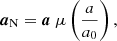
When solving the Jeans equation (Eq. (6)), the radial profile of the tracer number density is needed. We noted that for our galaxies the radial profiles of their GC surface number densities follow approximately a broken power law (see Fig. 1). We thus assumed that the GC volume number density has a form of
 |
Fig. 1. Surface-density profiles of the investigated GC systems. Points with error bars are measured data. Solid lines are fits by a broken power-law volume density profile (Eq. (2)). |
The free parameters of this model, the power-law exponents a and b, the normalization ρ0, and the break radius rbr, were obtained by fitting the data. For every galaxy we divided its GCs into several radial bins and calculated the surface density of GCs in each of the bins. We placed the bins so that each of them contained approximately the same number of GCs. The total number of bins was chosen individually for every galaxy by visual inspection so that both linear parts of the surface density profile were resolved by at least three points and, at the same time, the surface number density profile did not appear too noisy. We assumed that the survey that detected the GCs did so in a homogeneous way on our selected radial range. It is difficult to detect the GCs in the galaxy cores because of the galaxy glare. The innermost GCs were thus excluded if the surface-density profile appeared to deviate from the double power law profile in the galaxy center. In a few cases, we also noted a decline from the linear trend of the GC surface density profile at large radii, which we interpreted as a consequence of an incomplete GC survey in these distant areas. In these cases we excluded the most distant GCs until the surface density profile formed a single broken line. The volume number density given by Eq. (2) was converted to the surface number density numerically using the Abel transform. The parameter b was restricted to be b < −3 to ensure a finite number of GCs in the galaxies. In Table 2 we list for every galaxy the minimum and maximum radius of the GCs used (for all purposes in our paper), the number of such GCs, the number of bins used for obtaining the surface-density profiles, and the parameters of the best fits of the density profile. We note that the break radii expressed in kiloparsecs correlate with the stellar mass of the galaxy. This is similar to the behavior of effective radii of GC systems reported by Forbes (2017). This suggests that the breaks in the surface density profiles of the GC systems are physically real and do not result from some observational systematics. The systemic rotation velocities of the GC systems compiled from literature are included in Table 2.
The black points in panels a of Figs. C.1–C.20 show the projected radii and line-of-sight velocities of the GCs with the subtracted average radial velocities of the whole GC systems. We also plotted in those figures the corresponding velocity dispersion profiles (the green lines) and their uncertainty limits (the light green bands). The velocity dispersion and its uncertainty was calculated as
where N denotes the number of GCs in the bin, νi the radial velocity of the ith GC, and νsys the average line-of-sight velocity of all GCs in the galaxy. The bins had a variable width. Around each of the linearly spaced points where we wanted to calculate the velocity dispersion, we chose the bin edges such that they were symmetric around the point, there were at least 20 GCs between them, and the bin width that they defined was minimal but within the range of 0.5–4 Re.
The panels h and i of Figs. C.1–C.20 show the profiles of the s3 and s4 parameters (skewness and kurtosis, respectively) calculated in the same bins. These parameters are useful for constraining the anisotropy parameter β in the Jeans equation; see Sect. 4. The parameters quantify the deviation of the distribution from a Gaussian for which they are zero. A negative, zero, or positive kurtosis indicates tangential, isotropic, or radial orbits, respectively (Gerhard 1993). The kurtosis is however influenced by a systemic rotation of the GC system (Dekel et al. 2005). These parameters can be calculated as (Joanes & Gill 1998)
and
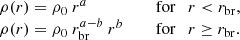
We also calculated these parameters for the whole GC systems assuming the velocity dispersion profile described above. The results are presented in Table 2. For all galaxies, the s4 parameter came out negative. This hints that the GCs are on tangential orbits. There are two pieces of evidence that this is a consequence of ordered rotation of the GC systems: First, the values of the s4 parameters anticorrelate with the average rotation velocity of the GC system, νrot, normalized by the total velocity dispersion of the GC system of the galaxy, σtot, as we can see in Fig. 2b. Second, the value of the s4 parameters anticorrelates with the rotator criterion number of the stars of the host galaxy (Sect. 8.1) so that the GC systems of fast-rotator galaxies have more negative values of the s4 parameter than the slow-rotator galaxies (Fig. 2a) and it was shown in the literature that the rotation of GCs, especially the red, correlates with the rotation of the stars of the host galaxy (Pota et al. 2013).
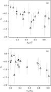 |
Fig. 2. Panel a: Kurtosis parameter s4 anticorrelates with the rotator criterion number of the host galaxy’s stars. Panel b: this parameter also anticorrelates with the average rotation velocity of the GC system normalized by the total velocity dispersion of the GC system galaxies. This suggests that the s4 parameter is driven by systemic rotation of the GC system. The host galaxies are distinguished by their environment (circles: field, triangles: group, asterisk: cluster). |
4. Solving the Jeans equation
Our study is based on comparing the observed radial velocities of the GCs to the theoretical models of line-of-sight velocity dispersion. The models of the latter were based on the spherically symmetric Jeans equation corrected approximately for systemic rotation (Binney & Tremaine 2008; Hui et al. 1995; Peng et al. 2004), i.e.,
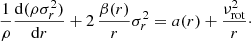
In this equation, r stands for the galactocentric distance and ρ(r) the number density of the GCs at r. The quantity σr(r) expresses the velocity dispersion in the direction toward the galaxy center. The value of velocity dispersion in the tangential direction, σt(r), enters the equation through the anisotropy parameter defined as  . This means that the GC orbits are predominantly radial if 0 < β ≤ 1, whereas for −∞≤β < 0 the GC orbits are predominantly tangential. The σr profile depends on the gravitational acceleration a(r) (having a negative sign). The term with the systemic rotation velocity νrot takes into account that the centrifugal force acts against the direction of gravity.
The radial velocity dispersion σr is not directly available from observations. Instead, we observe the line-of-sight velocities. The line-of-sight velocitity dispersion σlos at some projected galactocentric radius R is connected with σr through the equation (e.g., Binney & Mamon 1982)
![$$ \begin{aligned} \sigma _\mathrm{los} ^2(R) = \frac{\int _R^\infty \sigma _r^2(r)\, \left[ 1-(R/r)^2\beta \right]\, \rho (r)\, \left( r^2-R^2\right)^{-1/2}\,r\,\mathrm{d} r }{\int _R^\infty \rho (r)\, \left(r^2-R^2 \right)^{-1/2}\, r\, \mathrm{d} r }\cdot \end{aligned} $$](/articles/aa/full_html/2019/05/aa34675-18/aa34675-18-eq29.gif)
Having a model of the gravitational potential, the corresponding σlos profile can be determined using Eqs. (6) and (7). This requires solving a differential equation and calculating an integral at every R of interest, which is computationally demanding. Therefore we used the single-integral expression that was published by Mamon & Łokas (2005) for a few important profiles of the β parameter (their Eqs. (A15) and (A16)).
In order to test that our code calculates the profiles of σlos(R) correctly, we compared the outputs of our code to the known analytical solutions to Eqs. (6) and (7): the isotropic Hernquist sphere (Hernquist 1990); many forms of a power-law gravitational potential with a power-law tracer-density profile and a constant β; and the isotropic isothermal sphere (Binney & Tremaine 2008).
The velocity dispersion calculated using Eqs. (6) and (7) does not account for the fact that the observed velocity dispersion is increased by the systemic rotation of the GC system. We thus included the systemic rotation into the modeled line-of-sight velocity dispersion applying the usual approximation
which is the final expression we were using. We adopted the systemic rotation velocities of the GC systems for every galaxy from literature, see Table 2. We assumed that the GC systems rotate around an axis perpendicular to the line of sight and that the rotation velocities of all GCs around that axis are equal (see Côté et al. 2001 for a discussion of this common assumption).
The anisotropy parameter β remains unknown but certain restrictions follow from the values of the kurtosis parameter s4 discussed in Sect. 3. The proximity of the kurtrosis parameter for all our galaxies to zero (Sect. 3) led us to consider near-zero anisotropies. For every galaxy, we constructed models with the following types of anisotropy profile:
-
The isotropic profile following βiso = 0 at all radii
-
The mildly tangential profile with βneg = −0.5 at all radii
-
The “literature”, mildly radial profile βlit, given by the prescription,
where Re is the effective radius of the starlight of the galaxy (see below). With this profile, orbits are isotropic at the galaxy center and become tangential with β = 0.5 for radii large compared to Re. Such a profile is motivated by simulations of galactic mergers in ΛCDM (see Mamon & Łokas 2005 for details).
We considered the MOND and ΛCDM models. The choice of the gravity law then determines the acceleration field a in Eq. (6). The MOND acceleration a was determined from Eq. (1), in which we employed the interpolating function
The acceleration aN in Eq. (1) was calculated in the Newtonian way from the distribution of the visible matter as
where M*(< r) is the stellar mass cumulated below the radius r; i.e., we neglected, for example, the possible presence of interstellar gas. We assumed that the surface brightness of a galaxy follows the Sérsic profile (Sérsic 1963). This profile is characterized by the total luminosity L, the characteristic radius Re, and the Sérsic parameter n. We gathered these numbers for the photometric B band from literature; see Table 1. The mass-to-light ratio, M/L, is necessary to convert the luminosity surface density to the matter surface density. This ratio was one of the free parameters of our models. The mass cumulated interior to a given radius was obtained numerically by integrating the formula approximating the density profile of a Sérsic sphere by Lima Neto et al. (1999) with the update by Márquez et al. (2000).
Our ΛCDM models contained, apart from the stellar component, a NFW dark matter halo (Navarro et al. 1996). The mass of such a halo enclosed interior the radius r is
![$$ \begin{aligned} M_\mathrm{DM} ({<}r) = 4\pi \rho _{\rm s} r_{\rm s}^3\left\{ \ln \left[ \left(r_{\rm s}+r\right)/r_{\rm s}\right] - r/\left( r+r_{\rm s}\right) \right\} , \end{aligned} $$](/articles/aa/full_html/2019/05/aa34675-18/aa34675-18-eq34.gif)
where rs is the scale radius of the halo and ρs its scale density. Those were again treated as free parameters of the models. The gravitational field in the ΛCDM models is written as
![$$ \begin{aligned} a = -G\left[ M_*(<r)+M_\mathrm{DM} (<r)\right] /r^2. \end{aligned} $$](/articles/aa/full_html/2019/05/aa34675-18/aa34675-18-eq35.gif)
We identify in this paper the halo mass with the Mvir mass cumulated below the rvir radius. These quantities are defined according to Bryan & Norman (1998) so that we are consistent with the HMCR and SHMR definitions used by Diemer & Kravtsov (2015) and Behroozi et al. (2013), respectively.
5. Fitting the galaxy models
5.1. Methods
We compared the consistency of the observed line-of-sight velocities of the observed and simulated GCs with the expectations of ΛCDM and MOND in several ways. The approach described in this section consists in finding the best-fit parameters of the MOND and ΛCDM models of the galaxies, the results of which are then interpreted in Sect. 8. We determined the best values for the free parameters of the models using the maximum a posteriori approach, in which we maximize the product of the likelihood of obtaining the data if the parameters are given and the probability density of the parameters. Hereafter, when referring to GC radial velocities, we mean their measured radial velocities for which the average velocity of all the GCs was subtracted. We assumed that at a given galactocentric projected radius the distribution of GC radial velocities is Gaussian, has a zero mean and the velocity dispersion is determined by Eq. (8). Our priors on the free parameters were based on the independent estimates of the galaxy distances, stellar mass-to-light ratios, and the dark matter scaling relations, as we explain below. Let us denote the vector of the free parameters whose values are to be determined by the fit by p = (p1, p2, p3, …). Our next assumption was that the prior distributions of all the free parameters are Gaussian so that the distribution for the parameter pj has a mean of pj, exp and a standard deviation of Δpj. Let us further denote by σmod, i(p) the velocity dispersion implied by the parameters p at the radius of the ith GC and by νi the measured radial velocity of this GC. According to the maximum a posteriori method, we then have to find the parameters maximizing the function
We denoted the resulting parameters as  .
.
The free parameters are described below. All four of these parameters were used in the ΛCDM models while only the first two in the MOND models. Specifying these parameters is equivalent to specifying the galaxy distance, M/L, halo mass, and concentration, but the parameters we used are more advantageous for incorporating the prior knowledge and subsequently for interpreting the results. The free parameters were chosen so that the mean of the prior distribution of each pj, exp is zero.
-
The parameter pd expresses the deviation of the fitted distance d from the distance d0 measured by Tonry et al. (2001) on the basis of the surface-brightness fluctuations (see Sect. 2) as
The standard deviation of the prior distribution of this parameter, Δpd, follows straightforwardly from the uncertainty of the distance modulus given by Tonry et al. (2001).
-
We similarly introduced the parameter
to account for the uncertainty in the B-band M/L. Our prior knowledge of M/L follows from the star population synthesis models in Table 3. The expected value of M/L, M/L0, was chosen as log M/L0 = (log M/Lmin + log M/Lmax)/2, where M/Lmin and M/Lmax are, respectively, the minimum and maximum M/Ls listed for the particular galaxy in Table 3. We considered the standard deviation of the prior distribution for pM/L to be ΔpM/L = log M/Lmax − log M/L0.
-
The next parameter quantifies the deviation of the galaxy from the mean SHMR. We employed the formula for the mean SHMR by Behroozi et al. (2013). We adopted the same cosmological parameters as they did. Behroozi et al. (2013) concluded that the scatter of the stellar mass M* for a halo of a given mass Mh is Δlog M*(Mh) = 0.218 independently of Mh. Since our parameters pM/L and pd imply the value of M*, we had to invert this relation numerically and recover the scatter of Mh at a given M*, Δlog Mh(M*). It is then advantageous to quantify the deviation of the galaxy from the SMHR by the parameter
The expression Mh(M*) means the halo mass given by the Behroozi et al. (2013) SHMR formula and the stellar mass. The dispersion of the prior distribution of the parameter pSH is ΔpSH = 1.
-
The halo mass computed from the previous parameters implies a preferred halo concentration via the HMCR. For a given halo mass, we determined the concentration predicted by the HMCR using the COLOSSUS package for Python (Diemer 2018) assuming the HMCR function derived by Diemer & Kravtsov (2015). We benefited from the ability of COLOSSUS to calculate the HMCR function for any set of cosmological parameters. For a given halo mass Mh we defined
Diemer & Kravtsov (2015) found for isolated halos the scatter in the HMCR relation of 0.16 dex independently of Mh or redshift. An isolated halo is such that its center does not lie in the virial radius of another, larger halo. The dispersion of the prior distribution of the parameter pc is then Δpc = 0.16.

![$$ \begin{aligned} p_{\rm SH} = \frac{1}{\Delta \log M_{\rm h}(M_*)}\log \left[ \frac{M_{\rm h}}{M_{\rm h}(M_*)}\right]\cdot \end{aligned} $$](/articles/aa/full_html/2019/05/aa34675-18/aa34675-18-eq40.gif)
The 1σ uncertainty limits of the fitted value of the parameter pi can be determined by minimizing and maximizing pi over the region of the parameter space where

In order to calculate the 1σ uncertainty limits on some quantity A which is a function of p, we minimized or maximized A(p) over the same region. In Appendix B, we present a test of a correct recovering the free parameters from artificial data using these methods.
We rated the goodness of the fits in several ways: using the χ2 confidence, the corrected Akaike’s information criterion (AICc; Akaike 1974; Hurvich & Tsai 1989) and the logarithm of Bayes’s factor (LBF; Jeffreys 1961).
The χ2 statistics can be used to exclude a model as the only criterion out of the three. It is based on the fact that, for the correct model, the quantity
follows the χ2 statistical distribution with k degrees of freedom. The number of the degrees of freedom is the number of the fitted data points minus the number of the fitted parameters. In our case, k is therefore the number of the GCs. The models for which X2 lies in the tails of the corresponding χ2 distributions are considered excluded. We provide in Tables A.1 and A.2 the value of the confidence (conf.) of each model. It is the probability that a random number from the χ2 distribution has a larger deviation from the median of the distribution than X2. We considered the models with a confidence below 5% excluded; this is equivalent to a chi-square test with a 5% significance. This χ2 confidence allows an easier interpretation of the agreement of the model with the data than the traditional reduced χ2. If we had correct models for all our galaxies, then the fraction of galaxies with a confidence below x would be x.
The AICc and LBF criteria serve for determining which of several competing models matches the given observing data best. These criteria take into account the fact that the model with more free parameters is more likely to provide a better fit to the data. The AICc can be calculated as
where X2 is defined as above, k stands for the number of the fitted parameters (two for MOND or four for ΛCDM), and n for the number of data points (in our case the number of the GCs plus k). The model with the lowest AICc is preferred. This formula was derived with the assumptions that the model is linear in its free parameters and that the residuals from the fit follow a Gaussian distribution. The AICc criterion can thus give misleading results if systematic errors affect the measurement.
The LBF is defined as
![$$ \begin{aligned} \mathrm{LBF} = \log \int \mathcal{L} \left[\mathrm{data} |M(\boldsymbol{p})\right] f(\boldsymbol{p})\, \mathrm{d} \boldsymbol{p}. \end{aligned} $$](/articles/aa/full_html/2019/05/aa34675-18/aa34675-18-eq45.gif)
In this expression we integrate over the whole space of the free parameters. The term f(p) expresses the prior probability distribution function of p and ℒ[data|M(p)] the probability that the data is observed given that the model M holds true and has the free parameters p. If the portion of the parameter space that describes the data well is small, then the LBF comes out small. The LBF is a possible formalization of Occam’s razor. When comparing several models of the given data, that with the highest LBF is preferred. This parameter moreover does not require determining the number of free parameters of the model, which might be unclear in some cases (see Andrae et al. 2010 for examples). The price to pay is that the LBF is harder to calculate. We evaluated the integral in Eq. (22) using the Monte Carlo method. We generated 103 random realizations of p according to the prior distribution and then calculated 10LBF as the average of the corresponding values of ℒ, i.e., the first product in Eq. (14).
5.2. Resulting fits, comparing the ΛCDM and MOND models, dark halo scaling relations
Using the methods described above, we derived for every model the estimates and uncertainties of the quantities M/L, d, logρs and log rs. These values are stated for the ΛCDM and MOND models in Tables A.1 and A.2, respectively. In these tables we also provide the corresponding values of halo concentration c, rvir halo radius and Mvir mass, stellar mass M*, dark matter fractions (MDM/Mtot) interior to 1 and 5 Re,  and
and  , χ2 of the fit, and the statistical measures of the goodness of the fit, i.e., confidence, AICc, and LBF.
We can see that the ΛCDM models can describe all the galaxies successfully (the χ2 confidence is always higher than 5%). The worst cases are NGC 1023 and NGC 4494 with a confidence of approximately 38%. These galaxies require a weaker gravitational field than expected by the priors, as follows from panels b–e of Fig. C.2 and Fig. C.15. The ΛCDM models of these galaxies might require taking into account the rotation in the plane of the sky; see Sect. 8.
The MOND models were not successful for two galaxies of our sample (NGC 1399 and NGC 4486) meaning that the confidence of their best-fit models does not exceed 5% for any of the considered anisotropy profiles. We discuss the possible explanations is Sect. 8 (additional mass, another anisotropy parameter, and dynamical heating by neighboring galaxies).
Table 4 provides a comparison of the MOND and ΛCDM models for our galaxies in the terms of the AICc and LBF criteria. From all the considered anisotropy profiles, we show for every galaxy only the model that provides the best value of AICc or LBF. According to both AICc and LBF criteria, the MOND models are more successful for 9 out of the 17 real galaxies. If a ΛCDM model is preferred in some galaxy, then this preference is usually stronger than in the galaxies where a MOND model is preferred. The MOND models prefer mostly the βneg profile, while the ΛCDM prefer the βlit and βneg profiles in a comparable number of the real galaxies. Expectedly, the simulated galaxies R17x,y,z prefer mostly the βlit profile inspired by ΛCDM simulations.
Comparison of the best MOND and ΛCDM fits.
Our results also allow us to construct the SHMR and HMCR from the GC kinematics, which can be compared with theoretical expectations of the ΛCDM paradigm. The comparisons are presented in panels a and b of Fig. 3, respectively. The SHMR is presented in an equivalent form as the fitted baryonic fraction of the galaxy (i.e., the stellar mass divided by the halo mass) as a function of the halo mass. We can see that both the baryonic fraction and halo concentration indeed correlate tightly with the halo mass. We caution that the small scatter can be partly a consequence of our method, which disfavors deviations of the best-fit parameters from the theoretical correlations. The green lines denote the theoretical correlations and their scatter – that for the SHMR comes from Behroozi et al. (2013) and that for the HMCR from Diemer & Kravtsov (2015). Our recovered correlations deviate somewhat from the theoretical models. There are 14 galaxies out of the 17 lying above the mean theoretical SHMR. Using the binomial distribution, we can calculate that the probability that at least 14 galaxies out of 17 lie above the mean relation is 0.6%. For the HMCR, only 5 galaxies lie above the mean theoretical relation. Similarly, the probability that less than 5 of our galaxies lie above the theoretical relation is 2%. The deviations from both theoretical relations are thus statistically significant.
 |
Fig. 3. Panel a: stellar-to-halo mass relation. Symbols: recovered relation between the halo mass Mvir and the baryonic fraction in the halo M*/Mvir. Black symbols indicate real galaxies distinguished by environment (circles: field, triangles: group, asterisk: cluster). Blue symbols indicate the real galaxies dominating their environment clearly. Gray open stars indicate the galaxies R17x,y,z from a ΛCDM simulation. We show the parameters found for the anisotropy profile providing the best agreement with the GC data. The full green line indicates the theoretical SHMR found by Behroozi et al. (2013) based on the abundance matching technique. The dashed green lines denote the 1σ scatter region. The two real galaxies in the top left corner are NGC 1023 and NGC 4494. All individual galaxies agree with the prediction within the error bars but the reconstructed SHMR is offset. The collective offset does not seem to be substantially smaller for the dominant galaxies. Panel b: halo mass-concentration relation. The green lines indicate the theoretical HMCR by Diemer & Kravtsov (2015). The most outlying galaxy is NGC 4486. Again, the individual galaxies agree with the prediction but they are collectively offset from it, including the dominant galaxies. |
As explained below Eq. (20), if we had correct models of the GC kinematics for all our galaxies, then the fraction of galaxies with a confidence below x would be x because of the statistical noise. From this point of view, the ΛCDM models were too successful. From the models of 17 real galaxies, 15 of them could be fitted with the confidence value over 70%. As above, we can calculate that the probability that at least 15 out of 17 galaxy fits have a confidence over 70% is 1 × 10⁻⁴%. This probably means that the ΛCDM models are very flexible and fit even random noise in the data. On the other hand, the MOND models rather underfit the data since 11 out of the 17 galaxies have a confidence under 30% and the probability of obtaining at least this number of galaxy fits with a confidence below 30% is 0.32%.
We determined the characteristics of the galaxies with a low confidence of the MOND fits using the diagrams in Fig. 4 showing the confidence of the best-fit MOND model versus the given characteristic of the galaxy. If we had correct models of the data, the points would have the uniform distribution of the confidence. If the points concentrate toward a low value of confidence, this signifies an underfitting, i.e., the model does not capture the physical nature of the modeled system well. The concentration of the points toward high values of confidence rather signifies an overfitting of the data by the model. From these plots we can see that the confidence of the MOND fits decreases with an increasing stellar mass (as calculated assuming pd = pM/L = 0) for an increasing color index B − V, a decreasing ellipticity, a decreasing degree of rotational support of the galaxy λRe (Sect. 8.1), a decreasing rotator criterion number  (Sect. 8.1), and an increasing total kurtosis parameter of the GC system (as defined in Sect. 3). The decrease of the MOND confidence appears gradual for the degree of rotational support, λRe, and the kurtosis parameter of the GC system, s4. There seems to be a sudden drop of this confidence for the stellar mass above M* = 2.5 × 10¹¹ M⊙, the color index above B − V = 0.92, galaxy ellipticity below ϵ = 0.1, and the galaxy rotator criterion number below
  . Interestingly, there seems to be a sudden drop of the confidence of the best-fit MOND models at the value of the rotator criterion number separating the slow and fast rotators, which is indicated by the vertical dotted line in panel e of Fig. 4. The probability that all the 5 slow rotator best-fits have a confidence below 8% by coincidence is 3 × 10⁻⁴%.
 |
Fig. 4. Confidence of the best-fit MOND model depending on various properties of the galaxy. Panel a: stellar mass of the galaxy (derived for d0 and M/L0 defined in Sect. 5); panel b: color index B − V of the galaxy; panel c: galaxy ellipticity ϵ; panel d: degree of rotational support λRe (Eq. (24)); panel e: rotator criterion number |

As a check of the correctness of our method, we analyzed in the same way the artificial galaxies R17x,y,z. The values of M/L, d, log rs and logρs recovered using the GC kinematics (Table A.1) are all consistent with the true values (Sect. 2) within the 1 − 2σ uncertainty limits. This demonstrates that our method can recover the real parameters reasonably, at least for this particular simulated galaxy.
6. MOND and ΛCDM predictions of the velocity-dispersion profiles
In this section we compare the observed GC kinematics with the predictions of the ΛCDM and MOND paradigms. They were made without any fitting, just on the basis of independent estimates of the galaxy distances, luminosities, M/Ls, and the GC projected systemic rotation velocities. We assumed that the GC systems are kinematically isotropic. For the ΛCDM models, we further assumed that the galaxies follow the mean SHMR and HMCR relations. In other words, we set all of the parameters pi defined in Sect. 5 to zero.
The results are plotted in panels a of Figs. C.1–C.20 as the dotted lines: the blue lines correspond to the ΛCDM predictions and the red to the MOND predictions. We note several interesting points: (1) MOND usually underpredicts the observed velocity dispersion while ΛCDM usually overpredicts it. (2) ΛCDM always predicts a higher velocity dispersion than MOND. (3) The MOND predictions are almost always closer to the observed velocity-dispersion profile than the ΛCDM predictions or the goodness of the predictions appears comparable, i.e., MOND has a better predictive ability.
The last point is quantified in Fig. 5a where we calculated the RMS deviation of the predicted velocity dispersion profile, σlos, pred, from the observed velocity dispersion profile σlos, obs obtained in the way described in Sect. 3 (i.e., from the green curves in Figs. C.1–C.20) as ![$ \mathrm{RMS} = \left\{ n^{-1}\sum_{i=1}^n[\sigma_{\mathrm{los, pred}}(x_i) - \sigma_{\mathrm{los, obs}}(x_i)]^2\right\}^{1/2} $](/articles/aa/full_html/2019/05/aa34675-18/aa34675-18-eq51.gif) . The ratio of the RMS of the ΛCDM and MOND predictions is indeed mostly greater than one, which is shown by the black points. The red points demonstrate that the situation did not change appreciably even if we chose as the ΛCDM prediction3 the anisotropy profile out of βiso, βneg, and βlit individually for every galaxy so that the RMS deviation is minimized. The MOND predictions are in majority still better than the ΛCDM predictions even if the MOND models are put in disadvantage by substituting the real galaxy density distribution by a point mass that is shown in Fig. 5b by the black points or by the red points if optimized the ΛCDM prediction over the anisotropy profile.
. The ratio of the RMS of the ΛCDM and MOND predictions is indeed mostly greater than one, which is shown by the black points. The red points demonstrate that the situation did not change appreciably even if we chose as the ΛCDM prediction3 the anisotropy profile out of βiso, βneg, and βlit individually for every galaxy so that the RMS deviation is minimized. The MOND predictions are in majority still better than the ΛCDM predictions even if the MOND models are put in disadvantage by substituting the real galaxy density distribution by a point mass that is shown in Fig. 5b by the black points or by the red points if optimized the ΛCDM prediction over the anisotropy profile.
 |
Fig. 5. Panel a: comparison of the success of the predictions of the GC velocity dispersion profiles by MOND and ΛCDM. These predictions are based on independent estimates of the free parameters. The prediction assuming isotropy for both MOND and ΛCDM models are shown in black. The gray open stars represent the artificial galaxies R17x,y,z. It can be seen that MOND has a greater predictive ability. The same is true if the anisotropy model for the ΛCDM models is chosen out of the profiles βiso, βneg, and βlit so that it gives the lowest RMS, which is shown by the red points. Panel b: same but for the MOND prediction, the real galaxy density profiles were substituted by point masses. Despite this disadvantage, the MOND predictions still perform better, even if we again chose the anisotropy profile giving the best RMS for the ΛCDM. |
7. Radial acceleration relations
The RAR has been studied extensively in the LTGs but just a few studies have focused on the ETGs. In order to investigate the RAR on our data, we used special models of the gravitational field based on the ΛCDM models described in Sect. 5 so that the total gravitational field was approximated by a sum of the contribution from the stars and from a NFW halo. This is meant as a way to parametrize the gravitational field and therefore the values of fitted parameters could come out non-physical in the ΛCDM context. This form of gravitational field is justified by the fact that most rotation curves of the LTGs can be fitted well by a NFW halo. These models had three free parameters, the stellar M/L, which we allowed to be even negative, and the halo characteristic radius and density, which were both allowed to be only positive. In addition we required that the resulting gravitational field does not repel objects from the galaxy center on the radial range occupied by the GCs. The distance of the galaxies was set to be d0 (defined in Sect. 5). We checked that the gravitational fields expected by MOND for our galaxies can be approximated precisely in this way; the relative difference in the rotation curves could be made below 2% on the radial range occupied by the GCs. We obtained the best-fit parameters using the maximum likelihood method. This time, we did not use the priors on the free parameters so that we minimized only the first product in Eq. (14) because our goal was to fit the gravitational field as closely as possible. For every galaxy, we considered the three types of the anisotropy profiles described in Sect. 5.
For the best-fitting model, we evaluated the dynamical acceleration at ten galactocentric radii for every galaxy spaced logarithmically on the radial range occupied by the GCs. We found the uncertainty limits on these estimates using the method described in Sect. 5. The Newtonian accelerations aN were calculated assuming pM/L = pd = 0. The uncertainty of aN is written as
The results are plotted in panels f of Figs. C.1–C.20. We also plot by the gray band the RAR for the LTGs found by McGaugh et al. (2016). The thickness of the band corresponds to the 1σ scatter found in that study.
For most galaxies, at least one anisotropy profile allows a match with the LTG RAR within the 2σ uncertainty limit. The most discrepant objects are NGC 1399 and NGC 4486, which were already found to be inconsistent with MOND in Sect. 5.2. The objects for which we obtained the reconstructed dynamical acceleration, a, that is too low, NGC 1023 and particularly NGC 4494, might be quickly rotating in the plane of the sky. Another explanation is suggested by the simulated galaxies. Their reconstructed RARs deviate in a similar fashion. We know how quickly these galaxies rotate in all perpendicular projections. Since this rotation is not sufficient to explain the deviations and since the galaxies follow the LTG RAR (Sect. 2.2), these galaxies provide examples of how errors in the M/L and galaxy distance can affect the appearance of the RAR.
When all our RAR data points are put together, they broadly follow the RAR of the LTGs but with more scatter and the mean dynamical acceleration is higher at a given Newtonian acceleration; see Fig. 6. Its panel f indicates the error bars of the measured points obtained as the minimum and maximum a allowed by models with the three anisotropy profiles. We depicted in red the region covering the 1σ intrinsic scatter in the total RAR of ETGs determined using a maximum likelihood approach assuming that the average RAR does not change substantially over a 0.33 dex range in aN and that the total scatter is a combination of a Gaussian intrinsic scatter and a Gaussian scatter in the estimation of a. The 1σ scatter region of the LTG RAR (intrinsic scatter plus measurement error) as given by McGaugh et al. (2016) is denoted by the green boundary. The points in the other panels are colored with respect to various properties of the particular galaxies: the stellar mass (as determined assuming pd = pM/L = 0), galaxy color index B − V, galaxy ellipticity ϵ, galaxy degree of rotational support λRe (Eq. (24)), and the galaxy rotator criterion number  . We see a picture similar to the case with the fit confidence in Sect. 5.2: the deviation of the reconstructed RAR from that for the LTGs increases with a higher galaxy mass, redder color, decreasing support by rotation, and decreasing rotator criterion number.
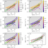 |
Fig. 6. Comparison of the RARs of the individual ETGs (colored points) and to the RAR of the LTGs (green region). The vertical thickness corresponds to the 1σ scatter (McGaugh et al. 2016). The points in panels a–e are colored with respect to the properties of their galaxy. Panel a – stellar mass of the galaxy (derived for d0 and M/L0 defined in Sect. 5); panel b – color index B − V of the galaxy; panel c – galaxy ellipticity ϵ; panel d – degree of rotational support λRe (Eq. (24)); panel e – rotator criterion number |

We verified the correctness of our method for reconstructing the RAR using the artificial galaxies R17x,y,z. The reconstructed data points indeed agree with the correct RARs (the orange dotted lines in panels f of Figs. C.18–C.20) within approximately 2σ uncertainty limits.
8. Discussion
8.1. Implications in the ΛCDM context
The GC systems have the advantage that they cover a substantial fraction of the dark halo. This helps when estimating the parameters of the halo. The scale radii of the NFW halos come out for LTGs typically five times their disk scale lengths (Navarro et al. 2017) while our most distant GCs lie further than 5 Re (see Figs. C.1–C.20). Our best-fit ΛCDM models confirm that the scale radii are often comparable to the extent of the GC system; see Table A.1.
We were able to find a statistically successful ΛCDM fit for every galaxy in the sample as determined using the chi-square test. The ΛCDM predictions on velocity dispersion are usually too high (Sect. 6). This is also the case of the galaxies NGC 1023 and NGC 4494 for which we obtained the worst ΛCDM models (confidence of around 38% for both). Statistical error can easily account for this confidence value. Nevertheless, the shape of the best-fit ΛCDM models for these galaxies seems to be too high for the outermost GCs (Figs. C.2 and C.13). The reason for this discrepancy might be the rotation of the GC system in the plane of the sky so that the attractive force is overestimated. This suggestion is supported by the fact that NGC 1023 and NGC 4494 have very low values of the s4 parameter among the real galaxies in our sample (Table 2) and as we showed in Sect. 3, this suggests a systemic rotation of the GC system. We can see in Table 2 that the systemic rotation of GC systems can exceed 100 km s−1. Future studies can use the rotation velocity in the plane of the sky as a free parameter.
Our galaxies form well-defined SHMR and HMCR relations (Fig. 3). We should remember that our method forces the best-fit models not to deviate substantially from the theoretical relations. Nevertheless, both of the recovered relations deviate from the theoretical expectations. In particular, most galaxies in the recovered HMCR relation lie below the relation deduced from cosmological dark-matter-only simulations of isolated halos by Diemer & Kravtsov (2015). We propose a few possible explanations. Some of our galaxies are not isolated, i.e., their center lies within a virial radius of another, more massive halo. Then this neighboring halo can tidally strip the outer part of the halo of the galaxy of interest and its concentration thereby decreases. In such a case, we expect that isolated galaxies and the galaxies dominating their environment would be affected the least. In order to test this idea, we chose the galaxies that are clearly dominant objects of their environment by visual inspection of the Digitized Sky Survey images using the Aladin software – NGC 821, NGC 1023, NGC 1399, NGC 1407, NGC 2768, NGC 3115, NGC 4472 and NGC 5128. These galaxies are denoted by the blue symbols in Fig. 3. The offset for the dominant galaxies does not seem to be substantially different than for the non-dominant sample. Another explanation might be that the ETGs prefer less concentrated halos than the LTGs that are missing in our sample, i.e. the result that our galaxies lie below the theoretical HMCR is a selection effect. This hypothesis could be investigated in existing cosmological hydrodynamical simulations or observationally using the rotation curves of the LTGs. The existing observational results suggest that the positions of the halos of the LTGs on the HMCR and SHMR depend on the assumed form of the halo and the priors (Katz et al. 2017; Li et al. 2019). On the other hand, the most luminous galaxies are nearly always ETGs, while our reconstructed HMCR deviates from the theoretical HMCR even for the most massive halos. The deviation of the recovered HMCR from the theoretical HCMR might also be caused by some systematic insufficiency of our ΛCDM models such as the plane-of-the-sky rotation of the GC system or some of the mechanisms suggested for the MOND models below. This kind of explanation seems inevitable for the extreme deviation of the galaxy NGC 4486 from the relation formed by the other galaxies. We should keep in mind a possible error in the theoretical HMCR.
We showed the SHMR as the baryonic fraction, log(M*/Mvir), as a function of the halo mass in Fig. 3a. The theoretical relation was based on abundance matching (Behroozi et al. 2013). The recovered relation is linear. Compared to the theoretical relation, the measured baryonic fraction in a halo is higher for a given halo mass and there is no turnover in the recovered relation near the halo mass of 1012 M⊙. We recall that three of the galaxies with log(M*/Mvir) > − 1.3 denoted by the open gray stars are the artificial galaxies R17x,y,z. The remaining two are NGC 1023 and NGC 4494. It is interesting that the RARs of these galaxies most clearly lie below the RAR of the LTGs; see panels f of Figs. C.1–C.20. Moreover, these galaxies have very low values of the s4 parameter (Table 2) among the sample and their chi-square confidences belong to the lowest. Interestingly, the artificial galaxies indicated by gray open stars have nearly the same fitted halo mass and the baryonic fraction, and we checked that these quantities were recovered correctly; the simulation that the galaxies come from was not designed to reproduce the SHMR. The same explanations of the deviation of the recovered HMCR from the theoretical HMCR apply for the SHMR apart from the fact that no assumption on galaxy isolation was made in the derivation of the theoretical SHMR (Behroozi et al. 2013).
We were interested in whether the velocity dispersion profiles of the artificial galaxies R17x,y,z were affected by the continual mergers that happen in a ΛCDM universe. To this end, we calculated the velocity dispersion profiles for the correct values of the galaxy distances, stellar masses, and dark halo parameters (Sect. 2.2). The galaxy Sérsic indices, effective radii, and GC rotation velocities were left as we derived them from the projected data (Tables 1 and 2). The results are indicated in panels a of Figs. C.18–C.20 by the orange dotted lines. A zero anisotropy was assumed. These theoretical profiles are well consistent with the measured profiles. This suggests that the GC kinematics was not affected by the mergers in this case. The galaxy in the simulation by Renaud et al. (2017) was relatively isolated and did not experience any major merger for 5 Gyr before the data were read, which means that the many subhalos moving through the GC system did not affect its kinematics substantially.
In the ΛCDM context, the apparent validity of MOND in the LTGs is considered a consequence of the profile of the dark halos, SHMR, HMCR, and the baryonic scaling relations (Di Cintio & Lelli 2016; Navarro et al. 2017). Interestingly, the MOND prescription (Eq. (1)) has a better predictive ability than the HMCR and SMHR, even if the MOND prediction is put at a disadvantage by substituting the galaxy by a point mass or optimizing the ΛCDM “prediction” over the anisotropy profile (Sect. 6). It might be again because we used a HMCR for isolated halos or because the halo shape also depends on the density distribution of the galaxy. The second point is probable because the MOND prescription works for the LTGs and there are pairs of LTGs with the same luminosity but very different rotation curves (the “Tully-Fisher pairs”; see, e.g., Sect. 4 of de Blok & McGaugh 1998).
We note that the degree of success of a MOND model of a GC system correlates with how much slow or fast rotator the host galaxy is. The slow and fast rotating ETGs can be distinguished observationally using integral field units. In these observations, we can introduce the degree of rotational support interior to 1 Re as
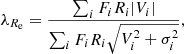
where we sum over the spaxels interior to 1 Re and Fi means the light flux from the spaxel, Ri its galactocentric radius, Vi the systemic velocity in the spaxel, and σi the velocity dispersion in the spaxel. The λRe parameter measures the degree of rotational support of the galaxy. The slow rotators are defined as the galaxies having the rotator criterion number  below 0.31, where ϵ is the ellipticity of the galaxy (Emsellem et al. 2011). Fast and slow rotators are two types of galaxies that have many contrasting properties. Most ETGs are fast rotators (86% according to Emsellem et al. 2011). We can use the rotator criterion number
  to quantify how fast or slow rotator a galaxy is. We found that this parameter correlates with the degree of success of the best MOND model of the galaxy measured by the chi-square confidence; see panel e of Fig. 4. Janz et al. (2016) noted that the dynamical masses of fast rotators determined from the GC kinematics using the tracer-mass-estimator method agree better with MOND than the dynamical masses of slow rotators. Similarly, Rong et al. (2018) found that the stellar kinematics of fast rotator ETGs is consistent with MOND while that of the slow rotators is less so. On the other hand, other observational evidence supports the validity of MOND even in slow rotators as we argue in Sect. 8.2. Our results suggest that in the ΛCDM context some connection between the degree of rotational support of the galaxy and its dark halo exists. Tenneti et al. (2018) detected a tight RAR for the rotationally supported galaxies in the MassiveBlack-II hydrodynamic cosmological simulation, which however differs from the RAR observed for the LTGs. It would be interesting to see whether the velocity-dispersion-supported galaxies in such simulations follow the same RAR and possibly spot the origin of the dependence on the galaxy rotation. Also, some of the explanations we suggest below for the MOND context could be true. However, most of these explanations cause an increase in velocity dispersion while the ΛCDM models in most galaxies already overpredict the velocity dispersion.
8.2. Implications in the MOND context
Our MOND models were not successful in two galaxies as determined by the chi-square test (NGC 1399 and NGC 4486, see Sect. 5.2). The AICc and LBF discriminators prefer the MOND models over the ΛCDM models in about a half of the galaxies but the preference is usually stronger for the ΛCDM models (Table 4). It is hard to decide whether this means that the ΛCDM paradigm is preferred over MOND based on our data alone because the assumed gravity prescription is just one of the uncertain ingredients of the models. The others include the anisotropy profile or the assumption of dynamical equilibrium, as described below. The following example demonstrates that the ΛCDM models are more likely to produce a better fit to the data even if some of the model assumptions are broken because of the higher flexibility of these models. We generated 100 radial profiles of the velocity dispersion for NGC 1399 with βiso, where we chose the pi parameters of the models randomly according to the prior statistical distributions (Sect. 5). The results are the blue curves in Fig. 7. We note that the most of these models follow the SHMR and HMCR well and are consistent with the observational constraints. The red curves in this figure were generated for the MOND models in the same way. The green curve is the observed velocity dispersion profile of NGC 1399. It is obvious that the ΛCDM models can provide a successful fit for a much larger variety of observed velocity dispersion profiles than the MOND models.
 |
Fig. 7. Demonstration that GC velocity dispersion profiles can be fitted easier by a ΛCDM model than by a MOND model even if the models omit some important aspect (e.g., halo stripping or perturbed GC kinematics). Blue lines indicate 100 random ΛCDM models of the velocity dispersion profile of NGC 1399, according to the statistical distribution of the free parameters described in Sect. 5. Such free parameters are well consistent with all the observational and theoretical constraints we have on the galaxy. Red lines indicate the same for the MOND models. Green line indicates the observed velocity dispersion profile of NGC 1399. |
If our MOND models were not successful for the slow rotator ETGs because MOND is invalid, then other tests of MOND in slow rotators based on independent methods should also be negative. The studies of stellar kinematics by Jeans analysis (e.g., Rong et al. 2018) are still similar to our method and could share the same weak points. Rong et al. (2018) might have come to their conclusion that the dynamical masses for the slow rotators are up to 60% higher than predicted by MOND because they used axially symmetric models for the galaxies, while most slow rotators exhibit more complex kinematics and misalignments between the kinematic and photometric axes (Emsellem et al. 2007, 2011; Graham et al. 2018). On the contrary, an independent method of measuring the gravitational field based on the requirement of hydrostatic equilibrium of the hot interstellar gas with gravity resulted in successful tests of MOND in slow rotators (Milgrom 2012; Lelli et al. 2017). We are not aware of a test of MOND by weak gravitational lensing specifically in slow rotators. Nevertheless, MOND was tested successfully in an “averaged” sample of red, presumably ETGs (Milgrom 2013). While most ETGs are fast rotators, the most massive ETGs are usually slow rotators; i.e., three-quarters above the stellar mass of 1011.5 M⊙ according to Emsellem et al. 2011 (see also Veale et al. 2017). There does not seem to be any indication of the deviation of the weak lensing data from the MOND prediction for the most massive galaxies (see Fig. 1 of Milgrom 2013). A dedicated test of MOND in slow rotators based on weak lensing would be welcome (Rong et al. 2018 had 144 slow rotators in their sample). Analysis of strong lensing by massive ETGs by Tian & Ko (2017) revealed that their dynamical masses agree with the MOND prediction and the interpolating function found for the LTGs. The small systematic deviation of around 20% could have easily been caused by a systematic error in the estimated stellar M/L. If MOND does not hold true in velocity-dispersion supported objects, it should be impossible to obtain satisfactory fits to the rotation curves of galaxies with dominant classical bulges. NGC 7814 has a classical bulge and bulge-to-total ratio of 0.85 (Bell et al. 2017). The rotation curve of this galaxy was fitted successfully in MOND (Angus et al. 2012b).
These facts led us to look for ways to explain the low success of some of our MOND models other than excluding MOND. These approaches are described in the following subsections. The MOND predicted velocity dispersions are usually lower than what is observed. The discrepancy probably has several sources. Some mechanisms to increase the velocity dispersion even more are necessary because of the external field effect: if the galaxy accelerates in an external gravitational field (such as from the galaxy cluster) its internal gravitational field is reduced in comparison to the galaxy being isolated (e.g., Milgrom 1983, 2014; Bekenstein & Milgrom 1984). In our models, the galaxies were treated as isolated. In the discussion below we assumed that the central galaxies of groups or clusters lie indeed in the geometrical centers of their environments and thus the external field effect is negligible.
8.2.1. Unaccounted matter
Our results could be explained by the presence of some mass component that we did not take into account. This contradicts some of the observations mentioned in the previous section but could be a viable option if substantial amounts of this material (say more than twice the stellar mass because of the uncertainty in the M/L in the above studies) are present just in a small fraction of galaxies, such as in the two most problematic galaxies NGC 1399 and NGC 4486. These are both central cluster galaxies whose GC systems extend over 100 kpc, therefore we might suspect the contribution of the hot intercluster gas is important. According to the observations of Paolillo et al. (2002), the mass of the X-ray emitting hot gas of NGC 1399 cumulated interior to 15′ is 1010 − 1011 M⊙. This is comparable to the stellar mass of the galaxy. Since the velocity dispersion in MOND scales with the fourth root of the baryonic mass, this contribution increases the velocity dispersion by around 20%, which is not enough. Such an increase would however be substantial for other galaxies, nevertheless exploring the mass of the interstellar gas in these galaxies is beyond the scope of this paper.
In NGC 1399, there seems to be several times more invisible matter than stellar matter as we can deduce either from the comparison of the MOND prediction on the velocity dispersion profile and the observed profile or from the comparison of the M/L of the best-fit MOND model of the galaxy and the SPS models. This has been already noted by Richtler et al. (2008) based on an analysis of the GC system of this galaxy. These authors suggested that this is a small scale version of the remaining missing mass problem of MOND in galaxy clusters. This MOND cluster-scale missing mass seems to form cores in galaxy cluster centers with characteristic radii of a few hundreds of kiloparcsec (Sanders 2003; Takahashi & Chiba 2007; Milgrom 2008). In the whole extents of galaxy clusters, MOND requires about as much of the invisible matter as baryonic matter. In galaxy cluster centers, the ratio of the invisible to visible mass increases up to the factor of a few. It is then expected that some of the invisible mass is also contained within the extents of the GC systems of the central cluster galaxies and thus the mass deficit in these galaxies does not pose an additional problem to MOND. The trend for slow rotators would be expected because they are mostly found in the cores of their clusters (Cappellari 2013; Houghton et al. 2013; D’Eugenio et al. 2013; Scott et al. 2014) because the slow rotator fraction increases with stellar mass and the most massive galaxies are found near galaxy cluster centers (Brough et al. 2017; Veale et al. 2017).
The following proposition adds to the “unaccounted matter” in a different way. Massive elliptical galaxies have a bottom-heavy IMF in their centers (Conroy & van Dokkum 2012). Thus, their M/L are higher than expected from the SPS models based on the IMF in the Milky Way or nearby galaxies. This might alleviate the deviation for our galaxies. van Dokkum et al. (2017) found that this change of the M/L is by a factor of 2.5 in galaxy centers but it decreases with radius so that the average M/L is enhanced by a factor of 1.3–1.5 at 1 Re. The fraction of stellar light enclosed in 1 Re is around 40% for our galaxies, thereby the total mass is increased by around 20%. This would help for some of the galaxies; compare Tables 3 and A.2. This correction would probably remove the small deviation in the strong lensing data from the MOND expectations in the work by Tian & Ko (2017).
8.2.2. GC systems out of dynamical equilibrium
Galaxy groups and clusters are dense environments where galaxies interact often. An encounter can dynamically heat the GC population. This would increase the velocity dispersion for a few dynamical times of the GC system until the system relaxes because of phase mixing (Mo et al. 2010). This explanation of the deviations from our MOND models appears very promising as we demonstrate on the example of NGC 4486 (=M 87), the central galaxy of the Virgo Cluster. The velocity field and galaxy distribution suggest that the center of this cluster is dynamically young and non-relaxed (Binggeli et al. 1987, 1993; Conselice et al. 2001; Lisker et al. 2018). A smaller galaxy cluster centered on M 86 is passing around the main core of the Virgo Cluster surrounding M 87. We can roughly estimate how much the velocity dispersion of the GCs around M 87 increased using the impulse approximation for high-speed encounters; i.e., we assume that the perturber moves with a constant velocity on a linear trajectory and the GCs do not move during the encounter. If the perturbing object has a mass of Mp, a velocity of νp, and the pericentric distance of the encounter is b, then the tidal force increases the velocity of a GC at distance of x from the center of M 87 by approximately (Mo et al. 2010)
If we substitute in this equation for νp the average velocity dispersion in the Virgo Cluster, 700 km s−1 (Binggeli et al. 1993), the dynamical mass of the M 86 subclump, Mp = 3 × 10¹³ M⊙ (Böhringer et al. 1994), the current projected distance of M 87 from M 86, d = 350 kpc, and x = 50 kpc for the characteristic distance of a GC, we obtain Δν = 150 km s−1. This would substantially alleviate the tension between the MOND models and the data, especially if the pericentric distance was closer than we used in this example. This is just a rough estimate and Eq. (25) should be adjusted for MOND, but this example already demonstrates the potential of galaxy encounters to increase the velocity dispersion of the GCs. These effects have to be studied using numerical simulations. In MOND this heating mechanism can be important since galaxies can have close encounters without ending in a merger because the dynamical friction is generally weaker in such configurations compared to Newtonian gravity with dark matter (Nipoti et al. 2007; Tiret & Combes 2008; Combes et al. 2010; Kroupa 2015; Renaud et al. 2016; Bílek et al. 2018) In other configurations, however the opposite can be the case (see Nipoti et al. 2008 for details). The signs of these encounters on the GC systems probably depend on the particular orbital geometry, masses of the galaxies, and orientation with respect to the observer. A close encounter with a pericenter closer than the extent of the GC system would probably cause asymmetries in the GC spatial distribution and kinematics. During more distant encounters, tidal torques would cause an increase of angular momentum of the corotating part of the GC population by the mechanism known to form tidal arms in spiral galaxies (see, e.g., Bournaud et al. 2010), which would induce systemic rotation of the GC system. The GC system would relax in a few dynamical times. We can estimate the dynamical time as 2πx/σtot, where σtot = 300 km s−1 stands for the typical observed velocity dispersion of the GCs around M 87 (Fig. C.2). The result is 1 Gyr. In this time, a galaxy with the average velocity equal to the velocity dispersion in the Virgo Cluster passes the path of 700 kpc. This is more than the observed projected distance to M 86 and it also is a substantial fraction of the size of the Virgo Cluster, meaning that many other galaxies could have perturbed the GC system. Interacting galaxies in MOND can reach a perhaps surprisingly large separation in 1 Gyr, even in sparse environments. In a self-consistent simulation reproducing the orbital history of the Local Group in MOND (Bílek et al. 2018), the Milky Way and Andromeda galaxies receded from the pericentric distance of about 25 kpc to about 600 kpc in 1 Gyr (see Fig. 5 there). Such close encounters probably affect the GC systems of galaxies substantially. Galaxy groups are also possibly an environment susceptible to disturbing the GC systems. They are often less dense than the clusters but the encounters have a lower relative speed.
There is more evidence that the galaxies in our sample experienced interactions apart from the high velocity dispersion of their GCs. We turn again to M 87 and M 86. These galaxies have approximately the same luminosity. If the smaller M 86 subclump increased the velocity dispersion of the GCs of M 87, then the GCs of M 86 had to be affected even more. According to Park et al. (2012), the velocity dispersion of the GCs of M 86 is virtually the same as that of M 87, around 300 km s−1. The average recession velocity of the GC system of M 86 is different from that of the M 86 core by over 100 km s−1, which can be a sign of tidal stripping. The isophotes of M 87 and its GC system are elongated approximately toward M 86 (Côté et al. 2001; Pota et al. 2013). The galaxy M 86 moves toward us with respect to the center of M 87, which is also the case of the GCs at M 87 at the side closer to M 86 (Côté et al. 2001; Pota et al. 2013). Regardless of the hypothesized influence of M 86, Murphy et al. (2014) showed that the stellar halo of M 87 is probably non-relaxed at the distance of 45 kpc from the galaxy center. Signs of galaxy interactions are detected in the kinematics of GCs and planetary nebulae of M 87 (Romanowsky et al. 2012; Longobardi et al. 2015). Some mechanism to explain the high concentration parameter is required for M 87 in the ΛCDM context as well (Fig. C.2).
Numerous signs of encounters exist in NGC 1399, the second of the two galaxies most problematic for our MOND models. Many of these signs have already been summarized in the GC review by Brodie & Strader (2006). This galaxy is the central galaxy of the Fornax Cluster. It has unusually many GCs for its luminosity while four other nearby galaxies have too few (Bassino et al. 2006a; Bekki et al. 2003). This suggests that the GCs were transferred from these smaller galaxies to NGC 1399. Such a transfer can be indeed achieved in simulations (Bekki et al. 2003). Additionally, the GCs of NGC 1399 have asymmetric spatial distribution (Bassino et al. 2006b) and kinematics (Richtler et al. 2004). Deep optical images of the Fornax Cluster show that the galaxies are connected by bridges of intracluster light and that one of these bridges is followed by an overdensity of the GCs of NGC 1399 (Iodice et al. 2017). This proves that the baryonic halo of this galaxy is not relaxed.
Signs of encounters have also been observed in other galaxies where the MOND models did not work very well. The galaxy NGC 4365 analyzed in this work still interacts with another galaxy, NGC 4342 (Blom et al. 2012a,b, 2014). There is an overdensity of GCs between the galaxies, which is aligned to the tidal features in NGC 4365. It was suggested that the GCs in this overdensity were stripped from NGC 4365. This would be supported by the fact that NGC 4365 (=VCC 731) has an unusually large amount of GCs for its luminosity (Peng et al. 2006). The alleged three-peaked color distribution of the GCs in NGC 4365 (e.g., Blom et al. 2012a) might be a consequence of the presence of GCs coming from NGC 4342 or another galaxy. The most obvious sign that NGC 4342 lost its outer parts because of the stripping is its central black hole, which is too massive for the stellar mass of the galaxy. This galaxy is an outlier from the relations between luminosity and effective radius, luminosity and metallicity, and luminosity and the central black hole mass (Blom et al. 2014). Galaxies with this mass of black hole of MBH = 108.7 M⊙ usually have a total stellar mass of around 1011 M⊙ (Reines & Volonteri 2015; Graham et al. 2016; Davis et al. 2018). This is a substantial fraction of the stellar mass of NGC 4365 (approximately 4 × 10¹¹ M⊙ according to Tables 1 and 3). Interestingly, Bogdán et al. (2012) excluded the possibility that NGC 4342 was tidally stripped because the analysis of the X-ray halo implies a high dynamical mass but the dark matter halo should have been stripped preferentially before the stars. This problem is removed by assuming MOND instead of a dark halo.
The fourth most discrepant galaxy, NGC 5846, possesses an asymmetric X-ray halo with sharp-edged structures that has been suggested to be a result of a galactic interaction (Machacek et al. 2011; Paggi et al. 2017). A suitable perturber could be the neighboring spiral galaxy NGC 5850 visible in Fig. C.17. Its strong bar and irregularities in spiral arms indicate that this galaxy interacted recently as well (Higdon et al. 1998).
Many signs of a strong interaction in NGC 5128 (=Cen A), whose RAR deviates noticeably from the RAR of the LTGs (panel f of Fig. C.16), are well known. These include the dust band (Quillen et al. 1993), stellar shells (Malin et al. 1983), or the twist in the velocity field of the planetary nebulae (Peng et al. 2004). The rotating disk of satellite galaxies detected at this galaxy by Müller et al. (2018) might be another sign. The best proposed mechanism to form such structures are galaxy encounters in which the satellites in the disks are tidal dwarf galaxies (Kroupa et al. 2005; Pawlowski et al. 2011, 2015; Fouquet et al. 2012; Kroupa 2015; Bílek et al. 2018; Banik et al. 2018). This would be supported by the fact that the satellites of Cen A seem to have a too high metallicity for their mass (Taylor et al. 2018) as if it was inherited from their mother galaxy. Malin et al. (1983) estimated that the time since the encounter is around 1 Gyr from the morphology of the dust lane and from the positions of the shells. The dynamical time of the GCs at Cen A at the galactocentric distance of 30 kpc is around 1 Gyr as well.
Galaxy encounters however also increase velocity dispersion in another way apart from tidal heating (Hilker et al. 2018). This mechanism is based on the fact that the baryonic halos of central cluster galaxies are grown by material released from the galaxies that fall on the central galaxy from the outskirts of the galaxy cluster or from the field. Because of the large difference of gravitational potential, the new GCs have a large velocity and increase the velocity dispersion of their new host substantially before the system relaxes dynamically. Employing this mechanism, Hilker et al. (2018) were able to explain the apparent disagreement of MOND with the stellar kinematics in the central galaxy of the Hydra I cluster, NGC 3311. This mechanism suggests itself particularly for the galaxies NGC 1399 and NGC 4365 showing multiple signs of capturing GCs of other galaxies.
When a galaxy moves through the galaxy cluster, its outskirts can also get out of dynamical equilibrium because of the varying external gravitational field via the MOND external field effect. This mechanism was studied recently by simulations (Candlish et al. 2018). The authors noted that the outskirts of the perturbed galaxy form a one-sided tail pointing in the direction away from the galaxy cluster center. We can then expect that this mechanism creates lopsided GC systems.
8.2.3. Other influences
Jeans analysis has a well-known difficulty with the anisotropy parameter. Its value is unknown and can vary within the volume of the galaxy. We noted that the degree of success of the MOND fits correlates with the degree of rotational support of the stellar component of the galaxy and with its rotator criterion number (panels d and e of Fig. 4). As we concluded in Sect. 3, more rotating galaxies have more rotating GC systems. This suggests that the degree of the rotational support of the GC system drives the success of the MOND fit. Since the support by random motion is weaker in rotating GC systems, a wrong anisotropy parameter or non-ordered motions are less important. This possibly partially explains why the GC systems of the fast rotators could be fitted by our MOND models better and also the results by Rong et al. (2018) that the kinematics of the stars of the fast rotators agrees better with MOND than that of the slow rotators. We recalculated our MOND predicted models from Sect. 6 for the βneg, βlit, and radial (β = 1) and nearly tangential (β = −20) anisotropy parameters. The parameter giving the highest velocity dispersion at large radii came out as nearly tangential. This provided velocity dispersion profiles increased by tens of km s−1 beyond 2 − 5 Re for all galaxies compared to the profiles calculated for the models with βiso.
Other mechanisms influencing the velocity dispersion include the following: the contamination of the GC population by the GCs moving in the total gravitational field of the cluster; the contamination by the GCs orbiting the satellite galaxies of the investigated galaxies; the presence of binary GCs, just as binary stars increase the observed velocity dispersion in dwarf galaxies (Dabringhausen et al. 2016); the anisotropic spatial distribution of GCs, such as that observed around the Milky Way (e.g., Pawlowski et al. 2012; Arakelyan et al. 2018); the substructures in the GC system resulting from stripping of other galaxies (e.g., like in NGC 3311, Hilker et al. 2018); or the systematic error introduced by our approximative treatment of the systemic rotation of the GC systems by Eq. (8).
An error in estimating the galaxy distance using the surface brightness fluctuation method could influence our results. We note that even a several-sigma deviation of the parameter pd from zero is actually not an extreme deviation in the distance itself. The greatest relative deviation of the best-fit distance to the prior estimate is 25% for the MOND models (NGC 1399) and 11% for the ΛCDM models (NGC 1407).
We should not forget the modified inertia versions of MOND in which the validity of Eq. (1) might be limited (Milgrom 1994, 2015). Unfortunately, no fully fledged modified inertia theory of MOND has been constructed yet.
9. Summary and conclusions
Gravitational fields of ETGs are difficult to investigate, especially at their outskirts (over a few effective radii, Re, of the galaxy’s stars) where the gravitational fields are expected to deviate substantially from the predictions of Newtonian dynamics without dark matter. The hypotheses proposed to explain the missing mass problem are thus tested poorly in ETGs. In this paper, we aimed to improve the situation and collected archival high-quality measurements of radial velocities of GCs in a sample of 17 ETGs. There were, in most cases, over 100 GC per galaxy. Such data have the advantage that the GCs often extend over 10 Re. The GC kinematics was investigated using the Jeans analysis. We focused on testing the predictions of the two most discussed propositions to solve the missing mass problem: the paradigms of the cold dark matter with a cosmological constant (ΛCDM) and MOND.
We investigated the gravitational fields in three ways. (1) We looked for the best-fit parameters of MOND and ΛCDM models of the GC kinematics using the Jeans equation and the maximum a posteriori fitting method (Sect. 5). The priors were an estimate of the galaxy distance, its stellar mass-to-light ratio (M/L) determined from the galaxy color, an estimate of the galaxy halo mass from the SHMR, and an estimate of the halo concentration from the HMCR. (2) We compared the observed velocity dispersion profiles to the predictions of MOND and ΛCDM supposing the galaxies follow the above-mentioned observational constraints and the mean HMCR and SHMR exactly (Sect. 6). (3) We constructed the RARs of the ETGs using a maximum likelihood approach (Sect. 7). Together with the real galaxies, we processed in the same way artificial data from a ΛCDM simulation of GC formation (Renaud et al. 2017), which helped with the interpretation of the results.
Successful ΛCDM fits were found for every galaxy in the terms of the chi-square test with a 5% significance level. The parameters of the best-fit models are presented in Table A.1. The GC systems analyzed in this work are advantageous for determining the halo parameters because the GCs often extend to a galactocentric radii comparable to the scale radii of the NFW dark halos. We compared the fit results with the theoretically predicted SHMR and HMCR (Fig. 3). The reconstructed points indeed show well-defined correlations in the SHMR and HMCR spaces and every individual galaxy agrees with the theoretical relations within the error bars. This might be partly because our fitting method disfavored deviations from the theoretical relations. Nevertheless, our recovered relations are offset from the theoretical relations. As for the HMCR, the real galaxies have a lower concentration for a given halo mass than predicted by Diemer & Kravtsov (2015) for isolated halos. A possible reason might be tidal stripping of the halos since most of our galaxies are not isolated, belonging to galaxy groups or clusters. We then expect the least deviations for the field galaxies and the central galaxies of groups and clusters. Another explanation might be that the ETGs reside in less concentrated halos than LTGs, i.e., that the offset of the reconstructed HMCR is a selection effect. This could be tested in cosmological hydrodynamical simulations or by a similar analysis of the rotation curves of the LTGs. The available facts nevertheless speak against both of these suggestions (Sect. 8.1). Comparing the reconstructed SHMR to the theoretical SHMR by Behroozi et al. (2013), our galaxies contain too much stellar mass for their halo masses. In addition, the reconstructed SHMR, if expressed as the baryonic fraction (i.e., the stellar mass divided by the halo mass) as a function of the halo mass, is linear and does not show the well-known maximum for the L* galaxies at the halo mass of around 1012 M⊙; however, this conclusion is based on just two data points, NGC 1023 and NGC 4494. The reason might again be halo stripping. We have to remember that all free parameters were fitted to the same data, and thus if the priors on one parameter are wrong, then all fitted parameters would be affected. The ΛCDM model usually predicts higher-than-observed GC velocity dispersion profiles (Sect. 6).
All but two galaxies could be fitted well by the MOND models according to the same test. The problematic cases are the central galaxies of the Fornax and Virgo clusters, NGC 1399 and NGC 4886, respectively. The success of the MOND fits generally decreases as the characteristics of the galaxies approach those found in the centers of galaxy groups or clusters (Fig. 4) because the GCs have an observed velocity dispersion that is too large (Sect. 8.2). A similar trend was found for the deviation of the RARs of our ETGs from the RAR of the LTGs, i.e., from the MOND prediction. It would not be surprising if these results were a consequence of a contribution of the additional dark matter that MOND requires in galaxy clusters: this dark matter is known to form cores of characteristic radii of a few hundreds of kiloparsecs (Sanders 2003; Takahashi & Chiba 2007; Milgrom 2008) and the extents of the GC systems are over 100 kpc for the most problematic galaxies (Sect. 8.2.1). Additionally, the dynamics of GCs of galaxies in dense environments is likely perturbed by galaxy interactions, which increase the velocity dispersion temporarily (Sect. 8.2.2). Indeed, we found many signatures of recent interactions or out-of-equilibrium GC systems in the most discrepant galaxies. Analytic estimates of the increase of the GC velocity showed that this proposition is promising, but simulations are necessary for a firmer conclusion.
We demonstrated that MOND is able to predict the velocity dispersion profiles in most ETGs better than ΛCDM even if the galaxies in the MOND models are approximated by point masses (Sect. 6). In the ΛCDM context, this probably means that the theoretical SHMR or HMCR we used should be updated for galaxies similar to those in our sample, for example, because dark halos are affected by tidal stripping. But then it is remarkable that MOND predicted the necessary direction of the correction.
Statistical criteria prefer MOND or ΛCDM models in a comparable number of galaxies: nine cases for MOND versus eight for ΛCDM, (see Table 4). The preference is however stronger in the cases where ΛCDM was preferred; thus ΛCDM emerged as the theory more suitable for describing our whole data set. This seems to be in a large part caused by the fact that the ΛCDM models are much more flexible than the MOND models. As we demonstrated in Fig. 7, if a galaxy is affected by some effect that we did not take into account, such as halo stripping or galaxy interactions, then a ΛCDM model is more likely to provide a better fit. This is supported by the fact that the ΛCDM fits had a high measure of success in a larger percentage of the galaxies than expected because of the statistical noise and this means that the ΛCDM models were even fitting noise in the data.
Acknowledgments
We thank Ivana Ebrová, Benedikt Diemer, and the anonymous referee for their valuable comments. SS acknowledges the support from the Ministry of Education, Science and Technological Development of the Republic of Serbia through project no. 176021 “Visible and Invisible Matter in Nearby Galaxies: Theory and Observations”. FR acknowledges support from the Knut and Alice Wallenberg Foundation. We acknowledge the usage of the HyperLeda database (http://leda.univ-lyon1.fr). This research has made use of “Aladin sky atlas” developed at CDS, Strasbourg Observatory, France. The Digitized Sky Surveys were produced at the Space Telescope Science Institute under US Government grant NAG W-2166. The images of these surveys are based on photographic data obtained using the Oschin Schmidt Telescope on Palomar Mountain and the UK Schmidt Telescope. The plates were processed into the present compressed digital form with the permission of these institutions. We acknowledge support provided by the European Commission through project BELISSIMA (BELgrade Initiative for Space Science, Instrumentation and Modelling in Astrophysics, call FP7-REGPOT-2010-5, contract no. 256772) in the early stage of this project.
References
- Akaike, H. 1974, IEEE Trans. Autom. Control, 19, 716 [NASA ADS] [CrossRef] [MathSciNet] [Google Scholar]
- Alabi, A. B., Forbes, D. A., Romanowsky, A. J., et al. 2017, MNRAS, 468, 3949 [NASA ADS] [CrossRef] [Google Scholar]
- Andrae, R., Schulze-Hartung, T., & Melchior, P. 2010, ArXiv e-prints [arXiv:1012.3754] [Google Scholar]
- Angus, G. W. 2008, MNRAS, 387, 1481 [NASA ADS] [CrossRef] [Google Scholar]
- Angus, G. W., van der Heyden, K. J., Famaey, B., et al. 2012a, MNRAS, 421, 2598 [NASA ADS] [CrossRef] [Google Scholar]
- Angus, G. W., van der Heyden, K. J., & Diaferio, A. 2012b, A&A, 543, A76 [NASA ADS] [CrossRef] [EDP Sciences] [Google Scholar]
- Arakelyan, N. R., Pilipenko, S. V., & Libeskind, N. I. 2018, MNRAS, 481, 918 [NASA ADS] [CrossRef] [Google Scholar]
- Arnold, J. A., Romanowsky, A. J., Brodie, J. P., et al. 2014, ApJ, 791, 80 [NASA ADS] [CrossRef] [Google Scholar]
- Banik, I., O’Ryan, D., & Zhao, H. 2018, MNRAS, 477, 4768 [NASA ADS] [CrossRef] [Google Scholar]
- Bassino, L. P., Richtler, T., & Dirsch, B. 2006a, MNRAS, 367, 156 [NASA ADS] [CrossRef] [Google Scholar]
- Bassino, L. P., Faifer, F. R., Forte, J. C., et al. 2006b, A&A, 451, 789 [NASA ADS] [CrossRef] [EDP Sciences] [Google Scholar]
- Begeman, K. G., Broeils, A. H., & Sanders, R. H. 1991, MNRAS, 249, 523 [NASA ADS] [CrossRef] [Google Scholar]
- Behroozi, P. S., Wechsler, R. H., & Conroy, C. 2013, ApJ, 770, 57 [NASA ADS] [CrossRef] [Google Scholar]
- Bekenstein, J., & Milgrom, M. 1984, ApJ, 286, 7 [NASA ADS] [CrossRef] [Google Scholar]
- Bekki, K., Forbes, D. A., Beasley, M. A., & Couch, W. J. 2003, MNRAS, 344, 1334 [Google Scholar]
- Bell, E. F., & de Jong, R. S. 2001, ApJ, 550, 212 [NASA ADS] [CrossRef] [Google Scholar]
- Bell, E. F., Monachesi, A., Harmsen, B., et al. 2017, ApJ, 837, L8 [NASA ADS] [CrossRef] [Google Scholar]
- Bender, R., Surma, P., Doebereiner, S., Moellenhoff, C., & Madejsky, R. 1989, A&A, 217, 35 [NASA ADS] [Google Scholar]
- Bílek, M., Ebrová, I., Jungwiert, B., Jílková, L., & Bartošková, K. 2015, Can. J. Phys., 93, iii [Google Scholar]
- Bílek, M., Cuillandre, J.-C., Gwyn, S., et al. 2016, A&A, 588, A77 [NASA ADS] [CrossRef] [EDP Sciences] [Google Scholar]
- Bílek, M., Thies, I., Kroupa, P., & Famaey, B. 2018, A&A, 614, A59 [NASA ADS] [CrossRef] [EDP Sciences] [Google Scholar]
- Binggeli, B., Tammann, G. A., & Sandage, A. 1987, AJ, 94, 251 [NASA ADS] [CrossRef] [Google Scholar]
- Binggeli, B., Popescu, C. C., & Tammann, G. A. 1993, A&AS, 98, 275 [NASA ADS] [Google Scholar]
- Binney, J., & Mamon, G. A. 1982, MNRAS, 200, 361 [NASA ADS] [CrossRef] [Google Scholar]
- Binney, J., & Tremaine, S. 2008, Galactic Dynamics, 2nd edn. (Princeton University Press) [Google Scholar]
- Blom, C., Spitler, L. R., & Forbes, D. A. 2012a, MNRAS, 420, 37 [NASA ADS] [CrossRef] [Google Scholar]
- Blom, C., Forbes, D. A., Brodie, J. P., et al. 2012b, MNRAS, 426, 1959 [NASA ADS] [CrossRef] [Google Scholar]
- Blom, C., Forbes, D. A., Foster, C., Romanowsky, A. J., & Brodie, J. P. 2014, MNRAS, 439, 2420 [NASA ADS] [CrossRef] [Google Scholar]
- Boch, T., & Fernique, P. 2014, in Astronomical Data Analysis Software and Systems XXIII, eds. N. Manset, & P. Forshay, ASP Conf. Ser., 485, 277 [NASA ADS] [Google Scholar]
- Bogdán, Á., Forman, W. R., Zhuravleva, I., et al. 2012, ApJ, 753, 140 [NASA ADS] [CrossRef] [Google Scholar]
- Böhringer, H., Briel, U. G., Schwarz, R. A., et al. 1994, Nature, 368, 828 [NASA ADS] [CrossRef] [Google Scholar]
- Bonnarel, F., Fernique, P., Bienaymé, O., et al. 2000, A&AS, 143, 33 [NASA ADS] [CrossRef] [EDP Sciences] [Google Scholar]
- Bournaud, F. 2010, in Galaxy Wars: Stellar Populations and Star Formation in Interacting Galaxies, eds. B. Smith, J. Higdon, S. Higdon, & N. Bastian, ASP Conf. Ser., 423, 177 [NASA ADS] [Google Scholar]
- Brada, R., & Milgrom, M. 1995, MNRAS, 276, 453 [Google Scholar]
- Brodie, J. P., & Strader, J. 2006, ARA&A, 44, 193 [NASA ADS] [CrossRef] [Google Scholar]
- Brough, S., van de Sande, J., Owers, M. S., et al. 2017, ApJ, 844, 59 [NASA ADS] [CrossRef] [Google Scholar]
- Bruzual, G., & Charlot, S. 2003, MNRAS, 344, 1000 [NASA ADS] [CrossRef] [Google Scholar]
- Bryan, G. L., & Norman, M. L. 1998, ApJ, 495, 80 [NASA ADS] [CrossRef] [Google Scholar]
- Candlish, G. N., Smith, R., Jaffé, Y., & Cortesi, A. 2018, MNRAS, 480, 5362 [NASA ADS] [CrossRef] [Google Scholar]
- Cappellari, M. 2013, ApJ, 778, L2 [NASA ADS] [CrossRef] [Google Scholar]
- Cappellari, M., Neumayer, N., Reunanen, J., et al. 2009, MNRAS, 394, 660 [NASA ADS] [CrossRef] [Google Scholar]
- Casuso, E., Vazdekis, A., Peletier, R. F., & Beckman, J. E. 1996, ApJ, 458, 533 [NASA ADS] [CrossRef] [Google Scholar]
- Ciotti, L., Londrillo, P., & Nipoti, C. 2006, ApJ, 640, 741 [NASA ADS] [CrossRef] [Google Scholar]
- Coccato, L., Gerhard, O., Arnaboldi, M., et al. 2009, MNRAS, 394, 1249 [NASA ADS] [CrossRef] [Google Scholar]
- Combes, F., & Tiret, O. 2010, in AIP Conf. Ser., eds. J. M. Alimi, & A. Fuözfa, 1241, 154 [Google Scholar]
- Conroy, C., & van Dokkum, P. G. 2012, ApJ, 760, 71 [NASA ADS] [CrossRef] [Google Scholar]
- Conselice, C. J., Gallagher, III, J. S., & Wyse, R. F. G. 2001, ApJ, 559, 791 [NASA ADS] [CrossRef] [Google Scholar]
- Côté, P., McLaughlin, D. E., Hanes, D. A., et al. 2001, ApJ, 559, 828 [NASA ADS] [CrossRef] [Google Scholar]
- Côté, P., McLaughlin, D. E., Cohen, J. G., & Blakeslee, J. P. 2003, ApJ, 591, 850 [NASA ADS] [CrossRef] [Google Scholar]
- Crain, R. A., Schaye, J., Bower, R. G., et al. 2015, MNRAS, 450, 1937 [NASA ADS] [CrossRef] [Google Scholar]
- Dabringhausen, J., Kroupa, P., Famaey, B., & Fellhauer, M. 2016, MNRAS, 463, 1865 [NASA ADS] [CrossRef] [Google Scholar]
- Davis, B. L., Graham, A. W., & Cameron, E. 2018, ApJ, 869, 113 [NASA ADS] [CrossRef] [Google Scholar]
- de Blok, W. J. G., & McGaugh, S. S. 1998, ApJ, 508, 132 [NASA ADS] [CrossRef] [Google Scholar]
- Dekel, A., Stoehr, F., Mamon, G. A., et al. 2005, Nature, 437, 707 [NASA ADS] [CrossRef] [PubMed] [Google Scholar]
- D’Eugenio, F., Houghton, R. C. W., Davies, R. L., & Dalla Bontà, E. 2013, MNRAS, 429, 1258 [NASA ADS] [CrossRef] [Google Scholar]
- De Vaucouleurs, G., Sandage, A., Sandage, M., & Kristian, J. 1975, Stars Stellar Systems, 9, 557 [Google Scholar]
- Di Cintio, A., & Lelli, F. 2016, MNRAS, 456, L127 [NASA ADS] [CrossRef] [Google Scholar]
- Diemer, B. 2018, ApJS, 239, 35 [NASA ADS] [CrossRef] [Google Scholar]
- Diemer, B., & Kravtsov, A. V. 2015, ApJ, 799, 108 [NASA ADS] [CrossRef] [Google Scholar]
- Dirsch, B., Richtler, T., Geisler, D., et al. 2003, AJ, 125, 1908 [NASA ADS] [CrossRef] [Google Scholar]
- Dullo, B. T., & Graham, A. W. 2014, MNRAS, 444, 2700 [NASA ADS] [CrossRef] [Google Scholar]
- Ebrová, I., Jílková, L., Jungwiert, B., et al. 2012, A&A, 545, A33 [NASA ADS] [CrossRef] [EDP Sciences] [Google Scholar]
- Emsellem, E., Cappellari, M., Krajnović, D., et al. 2007, MNRAS, 379, 401 [NASA ADS] [CrossRef] [Google Scholar]
- Emsellem, E., Cappellari, M., Krajnović, D., et al. 2011, MNRAS, 414, 888 [NASA ADS] [CrossRef] [Google Scholar]
- Famaey, B., & McGaugh, S. S. 2012, Liv. Rev. Relat., 15, 10 [Google Scholar]
- Fioc, M., & Rocca-Volmerange, B. 1997, A&A, 326, 950 [NASA ADS] [Google Scholar]
- Forbes, D. A. 2017, MNRAS, 472, L104 [NASA ADS] [CrossRef] [Google Scholar]
- Forbes, D. A., Alabi, A., Brodie, J. P., et al. 2017, AJ, 153, 114 [NASA ADS] [CrossRef] [Google Scholar]
- Fouquet, S., Hammer, F., Yang, Y., Puech, M., & Flores, H. 2012, MNRAS, 427, 1769 [NASA ADS] [CrossRef] [Google Scholar]
- Genel, S., Vogelsberger, M., Springel, V., et al. 2014, MNRAS, 445, 175 [Google Scholar]
- Gentile, G., Famaey, B., & de Blok, W. J. G. 2011, A&A, 527, A76 [NASA ADS] [CrossRef] [EDP Sciences] [Google Scholar]
- Gerhard, O. E. 1993, MNRAS, 265, 213 [NASA ADS] [CrossRef] [Google Scholar]
- Graham, A. W., Ciambur, B. C., & Soria, R. 2016, ApJ, 818, 172 [NASA ADS] [CrossRef] [Google Scholar]
- Graham, M. T., Cappellari, M., Li, H., et al. 2018, MNRAS, 477, 4711 [NASA ADS] [CrossRef] [Google Scholar]
- Harris, G. L. H. 2010, PASA, 27, 475 [NASA ADS] [CrossRef] [Google Scholar]
- Hernquist, L. 1990, ApJ, 356, 359 [NASA ADS] [CrossRef] [Google Scholar]
- Higdon, J. L., Buta, R. J., & Purcell, G. B. 1998, AJ, 115, 80 [NASA ADS] [CrossRef] [Google Scholar]
- Hilker, M., Richtler, T., Barbosa, C. E., et al. 2018, A&A, 619, A70 [NASA ADS] [CrossRef] [EDP Sciences] [Google Scholar]
- Houghton, R. C. W., Davies, R. L., D’Eugenio, F., et al. 2013, MNRAS, 436, 19 [NASA ADS] [CrossRef] [Google Scholar]
- Hu, J. 2008, MNRAS, 386, 2242 [NASA ADS] [CrossRef] [Google Scholar]
- Hui, X., Ford, H. C., Freeman, K. C., & Dopita, M. A. 1995, ApJ, 449, 592 [NASA ADS] [CrossRef] [Google Scholar]
- Hurvich, C. M., & Tsai, C.-L. 1989, Biometrika, 76, 297 [CrossRef] [MathSciNet] [Google Scholar]
- Hwang, H. S., Lee, M. G., Park, H. S., et al. 2008, ApJ, 674, 869 [NASA ADS] [CrossRef] [Google Scholar]
- Into, T., & Portinari, L. 2013, MNRAS, 430, 2715 [NASA ADS] [CrossRef] [Google Scholar]
- Iodice, E., Spavone, M., Cantiello, M., et al. 2017, ApJ, 851, 75 [Google Scholar]
- Israel, F. P. 1998, A&ARv, 8, 237 [NASA ADS] [CrossRef] [Google Scholar]
- Janz, J., Cappellari, M., Romanowsky, A. J., et al. 2016, MNRAS, 461, 2367 [NASA ADS] [CrossRef] [Google Scholar]
- Jeffreys, H. 1961, MR0187257 [Google Scholar]
- Joanes, D. N., & Gill, C. A. 1998, J. R. Stat. Soc.: Ser. D (The Statistician), 47, 183 [CrossRef] [Google Scholar]
- Katz, H., Lelli, F., McGaugh, S. S., et al. 2017, MNRAS, 466, 1648 [NASA ADS] [CrossRef] [Google Scholar]
- Kaviraj, S., Laigle, C., Kimm, T., et al. 2017, MNRAS, 467, 4739 [NASA ADS] [Google Scholar]
- Khandai, N., Di Matteo, T., Croft, R., et al. 2015, MNRAS, 450, 1349 [NASA ADS] [CrossRef] [Google Scholar]
- Kim, J.-H., Ma, X., Grudić, M. Y., et al. 2018, MNRAS, 474, 4232 [NASA ADS] [CrossRef] [Google Scholar]
- Kissler-Patig, M., Kohle, S., Hilker, M., et al. 1997, A&A, 319, 470 [NASA ADS] [Google Scholar]
- Komatsu, E., Dunkley, J., Nolta, M. R., et al. 2009, ApJS, 180, 330 [NASA ADS] [CrossRef] [Google Scholar]
- Komatsu, E., Smith, K. M., Dunkley, J., et al. 2011, ApJS, 192, 18 [NASA ADS] [CrossRef] [Google Scholar]
- Kormendy, J., Fisher, D. B., Cornell, M. E., & Bender, R. 2009, ApJS, 182, 216 [NASA ADS] [CrossRef] [Google Scholar]
- Krajnović, D., Alatalo, K., Blitz, L., et al. 2013, MNRAS, 432, 1768 [NASA ADS] [CrossRef] [Google Scholar]
- Kroupa, P. 2001, MNRAS, 322, 231 [NASA ADS] [CrossRef] [Google Scholar]
- Kroupa, P. 2015, Can. J. Phys., 93, 169 [NASA ADS] [CrossRef] [Google Scholar]
- Kroupa, P., Theis, C., & Boily, C. M. 2005, A&A, 431, 517 [NASA ADS] [CrossRef] [EDP Sciences] [Google Scholar]
- Lauer, T. R., Faber, S. M., Gebhardt, K., et al. 2005, AJ, 129, 2138 [NASA ADS] [CrossRef] [Google Scholar]
- Lauer, T. R., Gebhardt, K., Faber, S. M., et al. 2007, ApJ, 664, 226 [NASA ADS] [CrossRef] [Google Scholar]
- Lee, M. G., Hwang, H. S., Park, H. S., et al. 2008, ApJ, 674, 857 [NASA ADS] [CrossRef] [Google Scholar]
- Lelli, F., McGaugh, S. S., Schombert, J. M., & Pawlowski, M. S. 2017, ApJ, 836, 152 [Google Scholar]
- Li, H., Gnedin, O. Y., Gnedin, N. Y., et al. 2017, ApJ, 834, 69 [NASA ADS] [CrossRef] [Google Scholar]
- Li, P., Lelli, F., McGaugh, S., & Schormbert, J. 2018, A&A, 615, A3 [NASA ADS] [CrossRef] [EDP Sciences] [Google Scholar]
- Li, P., Lelli, F., McGaugh, S. S., Starkman, N., & Schombert, J. M. 2019, MNRAS, 482, 5106 [NASA ADS] [CrossRef] [Google Scholar]
- Lima Neto, G. B., Gerbal, D., & Márquez, I. 1999, MNRAS, 309, 481 [NASA ADS] [CrossRef] [Google Scholar]
- Lisker, T., Vijayaraghavan, R., Janz, J., et al. 2018, ApJ, 865, 40 [NASA ADS] [CrossRef] [Google Scholar]
- Longobardi, A., Arnaboldi, M., Gerhard, O., & Mihos, J. C. 2015, A&A, 579, L3 [NASA ADS] [CrossRef] [EDP Sciences] [Google Scholar]
- Machacek, M. E., Jerius, D., Kraft, R., et al. 2011, ApJ, 743, 15 [NASA ADS] [CrossRef] [Google Scholar]
- Makarov, D., Prugniel, P., Terekhova, N., Courtois, H., & Vauglin, I. 2014, A&A, 570, A13 [CrossRef] [EDP Sciences] [Google Scholar]
- Malin, D. F., Quinn, P. J., & Graham, J. A. 1983, ApJ, 272, L5 [NASA ADS] [CrossRef] [Google Scholar]
- Mamon, G. A., & Łokas, E. L. 2005, MNRAS, 363, 705 [NASA ADS] [CrossRef] [Google Scholar]
- Márquez, I., Lima Neto, G. B., Capelato, H., Durret, F., & Gerbal, D. 2000, A&A, 353, 873 [NASA ADS] [Google Scholar]
- McGaugh, S. S., Lelli, F., & Schombert, J. M. 2016, Phys. Rev. Lett., 117, 201101 [NASA ADS] [CrossRef] [Google Scholar]
- Merritt, D. 1997, AJ, 114, 228 [NASA ADS] [CrossRef] [Google Scholar]
- Milgrom, M. 1983, ApJ, 270, 365 [NASA ADS] [CrossRef] [Google Scholar]
- Milgrom, M. 1994, Ann. Phys., 229, 384 [NASA ADS] [CrossRef] [Google Scholar]
- Milgrom, M. 2008, New Astron. Rev., 51, 906 [NASA ADS] [CrossRef] [Google Scholar]
- Milgrom, M. 2010, MNRAS, 403, 886 [NASA ADS] [CrossRef] [Google Scholar]
- Milgrom, M. 2012, Phys. Rev. Lett., 109, 131101 [Google Scholar]
- Milgrom, M. 2013, Phys. Rev. Lett., 111, 041105 [NASA ADS] [CrossRef] [Google Scholar]
- Milgrom, M. 2014, MNRAS, 437, 2531 [NASA ADS] [CrossRef] [Google Scholar]
- Milgrom, M. 2015, Can. J. Phys., 93, 107 [NASA ADS] [CrossRef] [Google Scholar]
- Milgrom, M. 2017, ArXiv e-prints [arXiv:1703.06110] [Google Scholar]
- Milgrom, M., & Sanders, R. H. 2007, ApJ, 658, L17 [NASA ADS] [CrossRef] [Google Scholar]
- Mo, H., van den Bosch, F. C., & White, S. 2010, Galaxy Formation and Evolution (Cambridge: Cambridge Univ. Press) [Google Scholar]
- Müller, O., Pawlowski, M. S., Jerjen, H., & Lelli, F. 2018, Science, 359, 534 [NASA ADS] [CrossRef] [Google Scholar]
- Murphy, J. D., Gebhardt, K., & Cradit, M. 2014, ApJ, 785, 143 [NASA ADS] [CrossRef] [Google Scholar]
- Navarro, J. F., Frenk, C. S., & White, S. D. M. 1996, ApJ, 462, 563 [NASA ADS] [CrossRef] [Google Scholar]
- Navarro, J. F., Benítez-Llambay, A., Fattahi, A., et al. 2017, MNRAS, 471, 1841 [NASA ADS] [CrossRef] [Google Scholar]
- Nieto, J.-L., Poulain, P., Davoust, E., & Rosenblatt, P. 1991, A&AS, 88, 559 [NASA ADS] [Google Scholar]
- Nipoti, C., Londrillo, P., & Ciotti, L. 2007, MNRAS, 381, L104 [Google Scholar]
- Nipoti, C., Ciotti, L., Binney, J., & Londrillo, P. 2008, MNRAS, 386, 2194 [NASA ADS] [CrossRef] [Google Scholar]
- Paggi, A., Kim, D.-W., Anderson, C., et al. 2017, ApJ, 844, 5 [NASA ADS] [CrossRef] [Google Scholar]
- Paolillo, M., Fabbiano, G., Peres, G., & Kim, D.-W. 2002, ApJ, 565, 883 [NASA ADS] [CrossRef] [Google Scholar]
- Park, H. S., Lee, M. G., & Hwang, H. S. 2012, ApJ, 757, 184 [NASA ADS] [CrossRef] [Google Scholar]
- Pawlowski, M. S., Kroupa, P., & de Boer, K. S. 2011, A&A, 532, A118 [NASA ADS] [CrossRef] [EDP Sciences] [Google Scholar]
- Pawlowski, M. S., Pflamm-Altenburg, J., & Kroupa, P. 2012, MNRAS, 423, 1109 [NASA ADS] [CrossRef] [Google Scholar]
- Pawlowski, M. S., Famaey, B., Merritt, D., & Kroupa, P. 2015, ApJ, 815, 19 [NASA ADS] [CrossRef] [Google Scholar]
- Peng, C. Y., Ho, L. C., Impey, C. D., & Rix, H.-W. 2002, AJ, 124, 266 [NASA ADS] [CrossRef] [Google Scholar]
- Peng, E. W., Ford, H. C., & Freeman, K. C. 2004, ApJ, 602, 685 [NASA ADS] [CrossRef] [Google Scholar]
- Peng, E. W., Jordán, A., Côté, P., et al. 2006, ApJ, 639, 95 [NASA ADS] [CrossRef] [Google Scholar]
- Pillepich, A., Springel, V., Nelson, D., et al. 2018, MNRAS, 473, 4077 [NASA ADS] [CrossRef] [Google Scholar]
- Pota, V., Graham, A. W., Forbes, D. A., et al. 2013, MNRAS, 433, 235 [Google Scholar]
- Quillen, A. C., Graham, J. R., & Frogel, J. A. 1993, ApJ, 412, 550 [NASA ADS] [CrossRef] [Google Scholar]
- Reines, A. E., & Volonteri, M. 2015, ApJ, 813, 82 [NASA ADS] [CrossRef] [Google Scholar]
- Renaud, F., Famaey, B., & Kroupa, P. 2016, MNRAS, 463, 3637 [NASA ADS] [CrossRef] [Google Scholar]
- Renaud, F., Agertz, O., & Gieles, M. 2017, MNRAS, 465, 3622 [NASA ADS] [CrossRef] [Google Scholar]
- Rest, A., van den Bosch, F. C., Jaffe, W., et al. 2001, AJ, 121, 2431 [NASA ADS] [CrossRef] [Google Scholar]
- Richtler, T., Dirsch, B., Gebhardt, K., et al. 2004, AJ, 127, 2094 [NASA ADS] [CrossRef] [Google Scholar]
- Richtler, T., Schuberth, Y., Hilker, M., et al. 2008, A&A, 478, L23 [NASA ADS] [CrossRef] [EDP Sciences] [Google Scholar]
- Richtler, T., Famaey, B., Gentile, G., & Schuberth, Y. 2011, A&A, 531, A100 [NASA ADS] [CrossRef] [EDP Sciences] [Google Scholar]
- Romanowsky, A. J., Strader, J., Brodie, J. P., et al. 2012, ApJ, 748, 29 [NASA ADS] [CrossRef] [Google Scholar]
- Rong, Y., Li, H., Wang, J., et al. 2018, MNRAS, 477, 230 [NASA ADS] [Google Scholar]
- Salpeter, E. E. 1955, ApJ, 121, 161 [Google Scholar]
- Samurović, S. 2014, A&A, 570, A132 [NASA ADS] [CrossRef] [EDP Sciences] [Google Scholar]
- Samurović, S. 2016a, Serbian Astron. J., 192, 9 [NASA ADS] [CrossRef] [Google Scholar]
- Samurović, S. 2016b, Ap&SS, 361, 199 [NASA ADS] [CrossRef] [Google Scholar]
- Samurović, S. 2017, Serbian Astron. J., 195, 9 [NASA ADS] [Google Scholar]
- Samurović, S., & Ćirković, M. M. 2008, A&A, 488, 873 [NASA ADS] [CrossRef] [EDP Sciences] [Google Scholar]
- Samurović, S., & Ćirković, M. M. 2009, Publications de l’Observatoire Astronomique de Beograd, 86, 341 [NASA ADS] [Google Scholar]
- Samurović, S., & Vudragović, A. 2019, MNRAS, 482, 2471 [NASA ADS] [CrossRef] [Google Scholar]
- Samurović, S., Vudragović, A., Jovanović, M., & Ćirković, M. M. 2014, Serbian Astron. J., 188, 29 [NASA ADS] [CrossRef] [Google Scholar]
- Sanders, R. H. 1996, ApJ, 473, 117 [NASA ADS] [CrossRef] [Google Scholar]
- Sanders, R. H. 2003, MNRAS, 342, 901 [NASA ADS] [CrossRef] [Google Scholar]
- Saxton, C. J., & Ferreras, I. 2010, MNRAS, 405, 77 [NASA ADS] [Google Scholar]
- Schuberth, Y., Richtler, T., Hilker, M., et al. 2010, A&A, 513, A52 [NASA ADS] [CrossRef] [EDP Sciences] [Google Scholar]
- Scott, N., Davies, R. L., Houghton, R. C. W., et al. 2014, MNRAS, 441, 274 [NASA ADS] [CrossRef] [Google Scholar]
- Sérsic, J. L. 1963, Boletin de la Asociacion Argentina de Astronomia La Plata Argentina, 6, 41 [Google Scholar]
- Spolaor, M., Forbes, D. A., Hau, G. K. T., Proctor, R. N., & Brough, S. 2008, MNRAS, 385, 667 [NASA ADS] [CrossRef] [Google Scholar]
- Takahashi, R., & Chiba, T. 2007, ApJ, 671, 45 [NASA ADS] [CrossRef] [Google Scholar]
- Taylor, M. A., Eigenthaler, P., Puzia, T. H., et al. 2018, ApJ, 867, L15 [NASA ADS] [CrossRef] [Google Scholar]
- Tenneti, A., Mao, Y.-Y., Croft, R. A. C., et al. 2018, MNRAS, 474, 3125 [NASA ADS] [CrossRef] [Google Scholar]
- Tian, Y., & Ko, C.-M. 2017, MNRAS, 472, 765 [NASA ADS] [CrossRef] [Google Scholar]
- Tiret, O., & Combes, F. 2008, in Formation and Evolution of Galaxy Disks, eds. J. G. Funes, & E. M. Corsini, ASP Conf. Ser., 396, 259 [NASA ADS] [Google Scholar]
- Tiret, O., Combes, F., Angus, G. W., Famaey, B., & Zhao, H. S. 2007, A&A, 476, L1 [NASA ADS] [CrossRef] [EDP Sciences] [Google Scholar]
- Tonry, J. L., Dressler, A., Blakeslee, J. P., et al. 2001, ApJ, 546, 681 [NASA ADS] [CrossRef] [Google Scholar]
- Tortora, C., Romanowsky, A. J., Cardone, V. F., Napolitano, N. R., & Jetzer, P. 2014, MNRAS, 438, L46 [NASA ADS] [CrossRef] [Google Scholar]
- van Dokkum, P., Conroy, C., Villaume, A., Brodie, J., & Romanowsky, A. J. 2017, ApJ, 841, 68 [NASA ADS] [CrossRef] [Google Scholar]
- Veale, M., Ma, C.-P., Greene, J. E., et al. 2017, MNRAS, 471, 1428 [NASA ADS] [CrossRef] [Google Scholar]
- Weijmans, A.-M., Krajnović, D., van de Ven, G., et al. 2008, MNRAS, 383, 1343 [NASA ADS] [CrossRef] [Google Scholar]
- Woodley, K. A., Gómez, M., Harris, W. E., Geisler, D., & Harris, G. L. H. 2010, AJ, 139, 1871 [NASA ADS] [CrossRef] [Google Scholar]
Appendix A: Additional tables
ΛCDM fits.
MOND fits.
Appendix B: Test of recovering of free parameters
We tested our method and codes for reconstructing the parameters of the gravitational potential from the GC radial velocities by applying these codes on artificial data generated especially for this purpose. We assumed that we have artificial observations of 10 galaxies for which the following independent estimates are available: distance of 20 Mpc, luminosity of 2 × 10¹² L⊙, M/L of 5, effective radius of 3 kpc, and a Sérsic index of 4. In order to take the observational errors into account in our test, we randomly assigned each artificial galaxy the “real” parameters so that the pi parameters followed the statistical distributions described in Sect. 5 with ΔpM/L = 0.15 and Δpd = 0.04. This defines the real parameters of a galaxy: its distance, M/L, and the halo parameters. Then we could generate a GC system for every galaxy. Its number density was always proportional to r−3.5 and it contained 200 members extending from 0.1 to 5 effective radii of the galaxy. The radial velocities were generated with a Gaussian distribution with a velocity dispersion calculated at every radius according to the solution to Eqs. (6)–(7). We assumed a zero anisotropy and no systemic rotation. We applied our code to these data and compared the recovered and real parameters. This is shown in Fig. B.1. In this figure the index T stands for the true value and the index R for the recovered value. We can see that the recovered values are always correct at least by an order of magnitude and that the estimated uncertainty limits are reasonable.
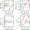 |
Fig. B.1. Test confirming that we can reconstruct the free parameters of the gravitational potential correctly from artificial data. The index “T” denotes the true value of the free parameter and “R” the reconstructed value. |
Appendix C: Results for individual galaxies
Panels a: Black points indicate galactocentric radii and absolute values of the radial velocities of the GCs. The systemic velocity of the whole GC system was subtracted. The galactocentric radius is expressed on the horizontal scale in the units of arcminutes, effective radii of the starlight of the galaxy, and kiloparsecs (assuming the mean distance from Table 2). The green line and band represent the running local line-of-sight velocity dispersion and its uncertainty (Sect. 3). The thick gray line indicates the line-of-sight velocity dispersion profile implied by the best-fit MOND model. The thick black line represents the same for ΛCDM. The dotted red line indicates the velocity dispersion profile predicted by MOND (Sect. 6). The dotted blue line indicates the same for ΛCDM. For the galaxies NGC 1407 and NGC 4472, the ΛCDM prediction lies outside the plot. The orange dotted lines in Figs. C.18–C.20 (R17x,y,z) represent the line-of-sight velocity dispersion profile calculated for a zero anisotropy and the correct parameters that these simulated galaxies have (Sect. 5.2). The red arrows indicate the radii where the acceleration calculated from the distribution of the stars in the Newtonian way (aN) reaches the quoted value (assuming the independent estimates of the galaxy distance and mass-to-light ratio).
Panels b–e: Comparison of the pi parameters expected for the galaxies from independent estimates (that we used as priors in Sect. 5) with the values we obtained by fitting the GC kinematics. The filled small black points with error bars represent the means and dispersions of the priors. The open gray points indicate the parameters of the best-fit MOND models. The open black points denote the same for the ΛCDM models.
Panels f: Gray band indicates the RAR for the LTGs reported by McGaugh et al. (2016) and its scatter. The colored points with error bars denote the RAR for our ETGs derived in Sect. 7. The color indicates the assumed anisotropy type (see Sect. 4).
Panels g: Image of the galaxy (prepared using the Aladin software (Bonnarel et al. 2000; Boch et al. 2014); the images come from the Digitized Sky Survey). North is up and east is left. The numbers stated in the middle of the bottom side show the size of the FOV. We chose the FOV so that its size is 3–4 times larger than the galactocentric distance of the furthermost GC. The size was increased (decreased) if there was (was not) another big galaxy nearby. In Fig. C.2 (NGC 4486), nearly all visible objects are galaxies.
Panels h and i show the radial profiles of the skewness (s3) and kurtosis (s4) parameters and their uncertainties, respectively (see Sect. 3). The plotted radial range matches that in the panel a. The horizontal dashed lines indicate the zero value.
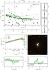 |
Fig. C.1. Results for the galaxy NGC 821. See page 26 for explanation. |
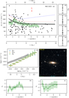 |
Fig. C.2. Results for the galaxy NGC 1023. See page 26 for explanation. |
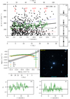 |
Fig. C.3. Results for the galaxy NGC 1399. See page 26 for explanation. |
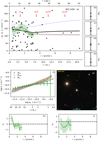 |
Fig. C.4. Results for the galaxy NGC 1400. See page 26 for explanation. |
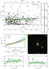 |
Fig. C.5. Results for the galaxy NGC 1407. See page 26 for explanation. The ΛCDM prediction in the panel a falls outside the plot. |
 |
Fig. C.6. Results for the galaxy NGC 2768. See page 26 for explanation. |
 |
Fig. C.7. Results for the galaxy NGC 3115. See page 26 for explanation. |
 |
Fig. C.8. Results for the galaxy NGC 3377. See page 26 for explanation. |
 |
Fig. C.9. Results for the galaxy NGC 4278. See page 26 for explanation. |
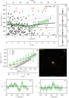 |
Fig. C.10. Results for the galaxy NGC 4365. See page 26 for explanation. |
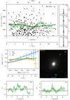 |
Fig. C.11. Results for the galaxy NGC 4472. See page 26 for explanation. The ΛCDM prediction in the panel a falls outside the plot. |
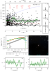 |
Fig. C.12. Results for the galaxy NGC 4486. See page 26 for explanation. |
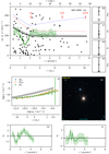 |
Fig. C.13. Results for the galaxy NGC 4494. See page 26 for explanation. |
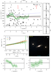 |
Fig. C.14. Results for the galaxy NGC 4526. See page 26 for explanation. |
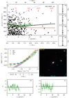 |
Fig. C.15. Results for the galaxy NGC 4649. See page 26 for explanation. |
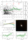 |
Fig. C.16. Results for the galaxy NGC 5128. See page 26 for explanation. |
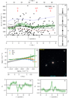 |
Fig. C.17. Results for the galaxy NGC 5846. See page 26 for explanation. |
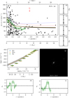 |
Fig. C.18. Results for the galaxy R17x. See page 26 for explanation. |
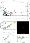 |
Fig. C.19. Results for the galaxy R17y. See page 26 for explanation. |
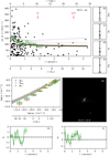 |
Fig. C.20. Results for the galaxy R17z. See page 26 for explanation. |
All Tables
All Figures
|
Fig. 1. Surface-density profiles of the investigated GC systems. Points with error bars are measured data. Solid lines are fits by a broken power-law volume density profile (Eq. (2)). |
| In the text | |
|
Fig. 2. Panel a: Kurtosis parameter s4 anticorrelates with the rotator criterion number of the host galaxy’s stars. Panel b: this parameter also anticorrelates with the average rotation velocity of the GC system normalized by the total velocity dispersion of the GC system galaxies. This suggests that the s4 parameter is driven by systemic rotation of the GC system. The host galaxies are distinguished by their environment (circles: field, triangles: group, asterisk: cluster). |
| In the text | |
|
Fig. 3. Panel a: stellar-to-halo mass relation. Symbols: recovered relation between the halo mass Mvir and the baryonic fraction in the halo M*/Mvir. Black symbols indicate real galaxies distinguished by environment (circles: field, triangles: group, asterisk: cluster). Blue symbols indicate the real galaxies dominating their environment clearly. Gray open stars indicate the galaxies R17x,y,z from a ΛCDM simulation. We show the parameters found for the anisotropy profile providing the best agreement with the GC data. The full green line indicates the theoretical SHMR found by Behroozi et al. (2013) based on the abundance matching technique. The dashed green lines denote the 1σ scatter region. The two real galaxies in the top left corner are NGC 1023 and NGC 4494. All individual galaxies agree with the prediction within the error bars but the reconstructed SHMR is offset. The collective offset does not seem to be substantially smaller for the dominant galaxies. Panel b: halo mass-concentration relation. The green lines indicate the theoretical HMCR by Diemer & Kravtsov (2015). The most outlying galaxy is NGC 4486. Again, the individual galaxies agree with the prediction but they are collectively offset from it, including the dominant galaxies. |
| In the text | |
|
Fig. 4. Confidence of the best-fit MOND model depending on various properties of the galaxy. Panel a: stellar mass of the galaxy (derived for d0 and M/L0 defined in Sect. 5); panel b: color index B − V of the galaxy; panel c: galaxy ellipticity ϵ; panel d: degree of rotational support λRe (Eq. (24)); panel e: rotator criterion number |
| In the text | |
|
Fig. 5. Panel a: comparison of the success of the predictions of the GC velocity dispersion profiles by MOND and ΛCDM. These predictions are based on independent estimates of the free parameters. The prediction assuming isotropy for both MOND and ΛCDM models are shown in black. The gray open stars represent the artificial galaxies R17x,y,z. It can be seen that MOND has a greater predictive ability. The same is true if the anisotropy model for the ΛCDM models is chosen out of the profiles βiso, βneg, and βlit so that it gives the lowest RMS, which is shown by the red points. Panel b: same but for the MOND prediction, the real galaxy density profiles were substituted by point masses. Despite this disadvantage, the MOND predictions still perform better, even if we again chose the anisotropy profile giving the best RMS for the ΛCDM. |
| In the text | |
|
Fig. 6. Comparison of the RARs of the individual ETGs (colored points) and to the RAR of the LTGs (green region). The vertical thickness corresponds to the 1σ scatter (McGaugh et al. 2016). The points in panels a–e are colored with respect to the properties of their galaxy. Panel a – stellar mass of the galaxy (derived for d0 and M/L0 defined in Sect. 5); panel b – color index B − V of the galaxy; panel c – galaxy ellipticity ϵ; panel d – degree of rotational support λRe (Eq. (24)); panel e – rotator criterion number |
| In the text | |
|
Fig. 7. Demonstration that GC velocity dispersion profiles can be fitted easier by a ΛCDM model than by a MOND model even if the models omit some important aspect (e.g., halo stripping or perturbed GC kinematics). Blue lines indicate 100 random ΛCDM models of the velocity dispersion profile of NGC 1399, according to the statistical distribution of the free parameters described in Sect. 5. Such free parameters are well consistent with all the observational and theoretical constraints we have on the galaxy. Red lines indicate the same for the MOND models. Green line indicates the observed velocity dispersion profile of NGC 1399. |
| In the text | |
|
Fig. B.1. Test confirming that we can reconstruct the free parameters of the gravitational potential correctly from artificial data. The index “T” denotes the true value of the free parameter and “R” the reconstructed value. |
| In the text | |
|
Fig. C.1. Results for the galaxy NGC 821. See page 26 for explanation. |
| In the text | |
|
Fig. C.2. Results for the galaxy NGC 1023. See page 26 for explanation. |
| In the text | |
|
Fig. C.3. Results for the galaxy NGC 1399. See page 26 for explanation. |
| In the text | |
|
Fig. C.4. Results for the galaxy NGC 1400. See page 26 for explanation. |
| In the text | |
|
Fig. C.5. Results for the galaxy NGC 1407. See page 26 for explanation. The ΛCDM prediction in the panel a falls outside the plot. |
| In the text | |
|
Fig. C.6. Results for the galaxy NGC 2768. See page 26 for explanation. |
| In the text | |
|
Fig. C.7. Results for the galaxy NGC 3115. See page 26 for explanation. |
| In the text | |
|
Fig. C.8. Results for the galaxy NGC 3377. See page 26 for explanation. |
| In the text | |
|
Fig. C.9. Results for the galaxy NGC 4278. See page 26 for explanation. |
| In the text | |
|
Fig. C.10. Results for the galaxy NGC 4365. See page 26 for explanation. |
| In the text | |
|
Fig. C.11. Results for the galaxy NGC 4472. See page 26 for explanation. The ΛCDM prediction in the panel a falls outside the plot. |
| In the text | |
|
Fig. C.12. Results for the galaxy NGC 4486. See page 26 for explanation. |
| In the text | |
|
Fig. C.13. Results for the galaxy NGC 4494. See page 26 for explanation. |
| In the text | |
|
Fig. C.14. Results for the galaxy NGC 4526. See page 26 for explanation. |
| In the text | |
|
Fig. C.15. Results for the galaxy NGC 4649. See page 26 for explanation. |
| In the text | |
|
Fig. C.16. Results for the galaxy NGC 5128. See page 26 for explanation. |
| In the text | |
|
Fig. C.17. Results for the galaxy NGC 5846. See page 26 for explanation. |
| In the text | |
|
Fig. C.18. Results for the galaxy R17x. See page 26 for explanation. |
| In the text | |
|
Fig. C.19. Results for the galaxy R17y. See page 26 for explanation. |
| In the text | |
|
Fig. C.20. Results for the galaxy R17z. See page 26 for explanation. |
| In the text | |
Current usage metrics show cumulative count of Article Views (full-text article views including HTML views, PDF and ePub downloads, according to the available data) and Abstracts Views on Vision4Press platform.
Data correspond to usage on the plateform after 2015. The current usage metrics is available 48-96 hours after online publication and is updated daily on week days.
Initial download of the metrics may take a while.