| Issue |
A&A
Volume 616, August 2018
|
|
|---|---|---|
| Article Number | A111 | |
| Number of page(s) | 12 | |
| Section | Interstellar and circumstellar matter | |
| DOI | https://doi.org/10.1051/0004-6361/201630316 | |
| Published online | 27 August 2018 | |
Extended ammonia observations towards the integral-shaped filament⋆
1
Xinjiang Astronomical Observatory, Chinese Acadmy of Sciences, Science 1-street 150, Beijing Road, Urumuqi, PR China
e-mail: wug@xao.ac.cn
2
School of Astronomy and Space Science, Nanjing University, 163 Xianlin Avenue, Nanjing, 210093, PR China
3
Key Laboratory of Radio Astronomy, Chinese Academy of Sciences, Urumqi, 830011, PR China
4
University of the Chinese Academy of Sciences, Beijing, 100080, PR China
5
Key Laboratory of Modern Astronomy and Astrophysics (Nanjing University), Ministry of Education, Nanjing 210023, China
6
Max-Planck-Institut für Radioastronomie, Auf dem Hügel 69, 53121 Bonn, Germany
7
Astronomy Department, King Abdulaziz University, PO Box 80203, Jeddah 21589, Saudi Arabia
Received:
22
December
2016
Accepted:
25
April
2018
Context. Recent observations suggest a scenario in which filamentary structures in the interstellar medium represent the first step towards clumps/cores and eventually star formation. The densest filaments would then fragment into prestellar cores owing to gravitational instability.
Aims. We seek to understand the roles filamentary structures play in high-mass star formation.
Methods. We mapped the integral-shaped filament (ISF) located at the northern end of the Orion A molecular cloud in NH3 (1, 1) and (2, 2). The observations were made using the 25 m radio telescope operated by the Xinjiang Astronomical Observatory, Chinese Academy of Sciences. The whole filamentary structure, about 1.2° × 0.6°, is uniformly and fully sampled. We investigate the morphology, fragmentation, kinematics, and temperature properties in this region.
Results. We find that the morphology revealed by the map of velocity-integrated intensity of the NH3 (1, 1) line is closely associated with the dust ridge revealed by the Herschel Space Observatory. We identify 6 “lumps” related to the well known OMC-1 to 5 and 11 “sub-clumps” within the map. The clumps and sub-clumps are separated not randomly but in roughly equal intervals along the ISF. The average spacing of clumps is 11.30′ ± 1.31′ (1.36 ± 0.16 pc) and the average spacing of sub-clumps is 7.18′ ± 1.19′ (0.86 ± 0.14 pc). These spacings agree well with the predicted values of the thermal (0.86 pc) and turbulent sausage instability (1.43 pc) by adopting a cylindric geometry of the ISF with an inclination of 60° with respect to the line of sight. We also find a velocity gradient of about 0.6 km s−1 pc−1 that runs along the ISF which likely arises from an overall rotation of the Orion A molecular cloud. The inferred ratio between rotational and gravitational energy is well below unity. Furthermore, fluctuations are seen in the centroid velocity diagram along the ISF. The OMC-1 to 5 clouds are located close to the local extrema of the fluctuations, which suggests that there exist gas flows associated with these clumps in the ISF. The derived NH3 (1, 1) and (2, 2) rotation temperatures in the OMC-1 are about 30–40 K while lower temperatures (below 20 K) are obtained in the northern and southern parts of the ISF. In OMC-2, OMC-3, and the northern part of OMC-4, we find higher and lower temperatures at the boundaries and in the interior, respectively.
Key words: ISM: clouds / ISM: structure / ISM: kinematics and dynamics / stars: formation / ISM: individual objects: ISF
The reduced data cubes are only available at the CDS via anonymous ftp to cdsarc.u-strasbg.fr (130.79.128.5) or via http://cdsweb.u-strasbg.fr/cgi-bin/qcat?J/A+A/616/A111
© ESO 2018
1. Introduction
In spite of the crucial role which high-mass stars (>8 M⊙) play in the evolution of the Universe, their formation and early evolution remains poorly understood (Zinnecker & Yorke 2007; Tan et al. 2014). High-mass stars always form in stellar clusters embedded in giant molecular clouds (GMCs). Recent observational studies reveal filamentary structures to be omnipresent in molecular clouds (e.g., André et al. 2010; Jackson et al. 2010; Li et al. 2014). Moreover, according to a “globular-filament” scenario of star formation (Schneider & Elmegreen 1979), filamentary structures in the interstellar medium represent the first step towards precluster clumps/prestellar cores and eventually star formation (André et al. 2014). The densest filaments would then fragment into clumps/cores owing to gravitational instability (e.g., Jackson et al. 2010).
Theories and models for filaments or gas cylinders have been studied for more than six decades (e.g., Chandrasekhar & Fermi 1953; Ostriker 1964; Inutsuka & Miyama 1992). The instability of gas cylinders shows some differences with respect to three-dimensional (3D) Jeans collapse. In a spherical gravitational Jeans collapse, perturbations of all wavenumbers grow at the same rate. However, in gas cylinders, perturbations of certain wavenumbers grow faster than others (Chandrasekhar & Fermi 1953; Jackson et al. 2010). Therefore, overdensities will tend to form at a length scale corresponding to this fastest growing wavenumber. Observationally, overdensities along filaments should be found at roughly regular intervals (the “sausage” instability; e.g., Jackson et al. 2010). Filaments are promising sites to study and test the physics of molecular cloud (MC) formation and fragmentation and to evaluate the earliest stages of high-mass star formation.
The Orion complex is the nearest and probably best studied on-going star formation region that continues to produce both low- and high-mass stars (Bally 2008). At a distance of about 414 ± 7 pc (Menten et al. 2007), it can be observed with good linear resolution even with a radio telescope of modest size. Meanwhile it is located about 15 degrees below the Galactic plane, leading to a less confused background than that typically encountered along the Galactic plane. Orion A is the largest MC (~31.5 deg2) in the Orion complex (Wilson et al. 2005). The integral-shaped filament (ISF) is the compact ridge at the northern end of the cometary Orion A cloud (Bally et al. 1987; Johnstone & Bally 1999). The ISF contains several clumps, namely OMC-1, OMC-2, OMC-3, OMC-4, and OMC-5 (e.g., Johnstone & Bally 1999, 2006). The ISF is an active high-mass star formation site and has spawned a sequence of stellar groups of different ages in the past few million years and likely contains hundreds of young stellar objects (Bally 2008).
To obtain physical information from the MCs, ammonia (NH3) inversion transitions are an invaluable spectroscopic tool due to the molecule’s lack of depletion, its hyperfine structure, and its sensitivity to kinetic temperature (Ho & Townes 1983). NH3 (1, 1) and (2, 2) have been proved to be an excellent thermometer under 20 K. It can also be a good thermometer for higher temperatures after some modification but with a reduction in precision (Walmsley & Ungerechts 1983; Danby et al. 1988; Tafalla et al. 2004). Moreover, the critical densities of NH3 (1, 1) and (2, 2) are about 103 cm−3 (Evans 1999; Shirley 2015), thus providing a proper tracer for the dense part of the filaments and their fragmentation.
In this paper, we therefore present uniform and fully sampled maps of the ISF in NH3 (1, 1) and (2, 2) and discuss the morphology, fragmentation, kinematics, and temperature properties in this region.
2. Observations and database archives
2.1. NH3 observations
The 25 m radio telescope, operated by the Xinjiang Astronomical Observatory, Chinese Academy of Sciences, was used for all the NH3 (1, 1) and (2, 2) observations presented here. The rest frequency was set at 23.708564 GHz for observing NH3 (1, 1) at 23.694495 GHz and NH3 (2, 2) at 23.722633 GHz, simultaneously. At this frequency, the telescope has a primary beam width (FWHM) of 125″ obtained from point-like continuum calibrators and a velocity resolution of 0.098 km s−1 provided by an 8192 channel Digital Filter Bank in a 64 MHz bandwidth mode. All line intensities reported here are in units of main beam brightness temperature Tmb.  values were calibrated against periodically (6 s) injected signals from a noise diode. Due to a hardware problem, we additionally used GBT (Green Bank Telescope) NH3 (1, 1) data (Friesen et al. 2017) to calibrate the spectra to the Tmb scale with ∼14% accuracy; see Appendix A.
The telescope pointing and tracking accuracy is better than 18″. A 22–24.2 GHz dual polarization channel superheterodyne receiver was used as frontend. On a  scale, the typical system temperature is about 50 K at 23 GHz. The map was made using the on-the-fly (OTF) mode with 6′ × 6′ grid size and 30″ sample step. All the observations were carried out in January 2014 under excellent weather conditions and above an elevation of 20°.
2.2. Archival data
The Herschel Space Observatory’s 100 μm, 250 μm, and 500 μm images using SPIRE/PACS parallel scan mode data were taken by Stutz & Kainulainen (2015). The PACS data and SPIRE data used here are level 2.5 products produced by the Herschel interactive processing environment (HIPE) software, version 12.1 (Ott 2010). The Montage1 and APLpy toolkits were used for cutout and plotting.
The archival 13CO spectra were observed with the IRAM 30 m telescope at Pico Veleta, Spain, in March, April, and October 2008. The data were obtained with the HEterodyne Receiver Array (HERA, 9 dual polarisation pixels arranged in the form of a 3 × 3 array with 24″ spacing) with an individual beam width of about 11″. The main beam efficiency at 220.4 GHz was 0.545. The VErsatile Spectrometric and Polarimetric Array (VESPA) was used as backend providing 320 kHz wide channels, which corresponds to roughly 0.4 km s−1. The map was made in the on-the-fly (OTF) mode, with 5″ data sampling in right ascension, and with steps of 12″ in declination. The rms per channel is about 0.2 K on a main beam brightness temperature scale (for more details, see Berné et al. 2014).
3. Data reduction and results
The CLASS and GREG packages of GILDAS2, and also python plot packages matplotlib (Hunter 2007) and APLpy3 were used for all the data reduction. Second-order polynomial fitting is used for baseline removal and the mean rms per channel is about 0.3 K on a main beam brightness temperature scale. In order to convert hyperfine blended line widths to intrinsic line widths in the NH3 inversion spectrum (e.g., Barranco & Goodman 1998), we fitted the averaged spectrum using the GILDAS built-in “NH3 (1, 1)” fitting method which can fit all 18 hyperfine components simultaneously.
The NH3 (1, 1) and (2, 2) velocity-integrated line intensity (zeroth moment) maps are presented as gradations of gray-scale intensities and contours in Fig. 1. The integration range is from 6.5 to 12.5 km s−1 to cover the main group of hyperfine components (△F = 0, Ho & Townes 1983) of the NH3 (1, 1) or (2, 2) transitions. We adopt this integration range since in relatively diffuse parts of the ISF, where NH3 is barely detectable, the satellite lines (△F = ±1, Ho & Townes 1983) are usually not accessible and the velocity integrated intensity including satellite lines would lead to lower signal-to-noise ratios (S/Ns). Meanwhile, we also constructed a velocity integrated intensity image including all hyperfine components (the main group and the four groups of satellite lines). The morphology, especially in the denser regions, is similar to the image only including the main line. Furthermore, the results related to clump and sub-clump identification (Sect. 4.1) are not changed.
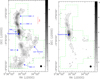 |
Fig. 1. Integrated intensity (zeroth moment) maps of NH3 (1, 1) (left) and (2, 2) (right). The integration range of each panel is 6.5 < VLSR < 12.5 km s−1. Contours start at 0.96 K km s−1 (4σ) on a main beam brightness temperature scale and go up in steps of 0.96 K km s−1. The limits of the mapped region are indicated with green dashed lines. A blue star in each panel indicates the Trapezium cluster and black filled circles in the lower right illustrate the half-power beam size. |
In Fig. 1, contours start at 0.96 K km s−1 (4σ, thick gray line) and go up in steps of 0.96 K km s−1 (thin gray lines). σ is equal to  , where rms is the averaged baseline channel rms of all spectra exported from the baseline fitting with CLASS (being part of the GILDAS package), V is the channel spacing, and N_channels is the channel number in the integrated velocity range (6.5–12.5 km s−1). In each panel, the Trapezium cluster is labeled as a blue star and the half-power beam width is illustrated as a black filled circle in the lower right bottom. The limits of the mapped region are indicated with green dashed lines. The clumps OMC-1 to 5 are labeled in the left panel. The red line in the top right of the left panel illustrates the 1 pc scale at a distance of 414 pc (Menten et al. 2007). An additional “sub filament” structure in the west of OMC-4 is also labeled in the left panel. The whole map consists of a total of 45 240 raw spectra. After smoothing to 1′ × 1′ areas, 1764 uniformly spaced spectra remain, covering a region about 1.2 degrees in declination and about 0.6 degrees in right ascension.
In the left panel of Fig. 1, the zeroth moment map of NH3 (1, 1) shows an integral-shaped morphology (∫) as observed in 13CO (see Bally et al. 1987). Compared to 13CO, NH3 (1, 1) highlights the main filamentary structure and the fragmentation in a clearer way and we find, unlike what is seen in 13CO, little diffuse gas around the ISF. In NH3 (1, 1), the length of the ISF is about 7 pc, and the width is about 1 pc at a distance of 414 pc. The densest regions all show elongated morphologies, mainly along the main axis of the ISF, hinting at the existence of sub-structures which are displayed in more detail in Fig. 7 of Friesen et al. (2017). A separated emission region located between the OMC-1 and the already mentioned western sub-filament is not analysed in this work, since only a few pixels show NH3 (1, 1) detections in this region. According to the right panel of Fig. 1, most of the NH3 (2, 2) line detections are obtained in the northern part of the ISF. Considering weaker NH3 (1, 1) intensities in the southern part of the ISF (left panel of Fig. 1) and keeping in mind that CO is also weaker in the south (e.g., Bally et al. 1987; Wilson et al. 2005), this is likely caused by lower NH3 column densities in the southern part of the ISF.
4. Discussion
4.1. Ammonia morphology and two level fragmentation in the ISF
A false color Herschel infrared image of the ISF is shown in the left panel of Fig. 2 (red for 500 μm, green for 250 μm, and blue for 100 μm), overlaid with NH3 (1, 1) integrated intensity contours as in Fig. 1. From this panel, we can see the contours are closely associated with the dust ridge presented by the Herschel infrared emission. As mentioned in Sect. 3, there is a sub-filament in addition to the main filamentary structure, which is extruded in the west of OMC-4 and which is identified for the first time in NH3. The sub-filament has a length of about 20′, that is, about 2 pc at a distance of 414 pc. In the left panel of Fig. 2, there is also an obvious infrared feature corresponding to this sub-filament.
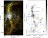 |
Fig. 2 Left panel: false color image of the ISF (red for 500 μm, green for 250 μm, and blue for 100 μm, all Herschel data) overlaid with NH3 (1, 1) integrated intensity contours, as in Fig. 1. Right panel: “clumps” and “sub-clumps” are labeled as red crosses and yellow filled circles, respectively, on the NH3 (1, 1) integrated intensity map. |
From the NH3 (1, 1) integrated intensity map, we find that the six regions with strongest NH3 emission are located along the ISF. In the right panel of Fig. 2, we marked the six regions (two related to OMC-4) with strongest NH3 emission as “clumps” with red crosses on the NH3 map. The emission peaks correspond to significant star-forming regions within the Orion A Molecular Cloud (e.g., Bally et al. 1987; Johnstone & Bally 1999, 2006). Following the terminology of Johnstone & Bally (1999, 2006), we name them OMC-1 to 5. Since the two regions in OMC-4 are separated by more than a typical clump size of 1 pc (e.g., hierarchical fragmentation in Zhang et al. 2009; Wang et al. 2014), we consider them as two separate “clumps”. These clumps are not randomly spaced but at roughly equal intervals. The average spacing of these five clumps is 11.30′ ± 1.31′ (given uncertainties are errors of the mean), that is, 1.36 ± 0.16 pc at a distance of 414 pc (Menten et al. 2007). We then used the Clumpfind2d algorithm (Williams et al. 1994) with a threshold of 5σ and increments of 2σ (σ is defined in Sect. 2.1) to identify sub-structure. Lu et al. (2014) and Ohashi et al. (2016), for example, used similar parameters to identify sub-structures. Eleven such sub-structures were identified within the NH3 map after excluding a fake one located at the boundary of the map. We also present the pixels used to define these sub-structures in Appendix B. As the sub-structures are smaller than 1 pc and larger than 0.1 pc, we name these sub-structures “sub-clumps”. Pineda et al. (2009) argued the specific selection of the parameters in the Clumpfind2d algorithm may result in slight differences in identifying the condensations, but it works well for relatively isolated sub-clumps which we find in the ISF. In our observation, the clumpfind2d algorithm is more sensitive to the threshold we have chosen, and not to the increments. Using a threshold of 3σ, the procedure tends to find some additional artificial condensations at the edge of the image. Therefore, we adopt a robust threshold of 5σ and increments of 2σ leading to an identification of those sub-clumps that one would tend to select by eye. We marked these sub-clumps as yellow filled circles in the right panel of Fig. 2. As we can see, the ten sub-clumps within the main structure of the ISF are also regularly separated. The average spacing is 7.18′ ± 1.19′, which corresponds to 0.86 ± 0.14 pc at 414 pc.
The results may suffer from the effect of the small number statistics. Before we interpret the results, we considered 1 million tests of six-element random arrays in the range of 0 to 1.36 × 6 pc. About 1.1% of these random arrays are more equally spaced (the ratio of the standard deviation of the mean to the mean value is less than 0.16 pc/1.36 pc). Subsequently, we considered 1 million tests of ten-element random arrays in the range of 0–0.86 × 10 pc. About 2.5% of these random arrays are more equally spaced (the ratio of the standard deviation of the mean to the mean value is less than 0.14 pc/0.86 pc).
The approximately equal intervals of the clumps can be explained by a so-called sausage instability firstly proposed by Chandrasekhar & Fermi (1953) for an incompressible gas cylinder. Following Jackson et al. (2010), for an isothermal cylinder with infinite radius, the characteristic length between adjacent condensations is about 22H. H is the isothermal scale height given by H = cs(4πGρc)−1/2, where cs is the sound speed, G is the gravitational constant, and, ρc is the gas mass density at the center of the filament. For an isothermal cylinder of finite radius R surrounded by an external, uniform medium, the characteristic length for R ≫ H is also about 22H. If R ≪ H, the characteristic length becomes about 11R.
We assumed the ISF is an isothermal cylinder with a typical kinetic temperature of 18 K (see Sect. 4.3) and a central volume average density of the ISF of 104 cm−3 (Bally et al. 1987; Cesaroni & Wilson 1994; Johnstone & Bally 1999). Then the sound speed  , taking μH = 2.4 and mH = 1.674 × 10⁻²⁴ g. The isothermal scale height is H ∼ 0.04 pc. Therefore, under the regimeR ≫ H,thecharacteristiclength(22H) of the ISF is about 1 pc. Assuming a median inclination of a randomly oriented filament of 60° with respect to the line of sight (Genzel & Stutzki 1989; Hanawa et al. 1993), the projected spacing will be 1 pc × sin(60°) ∼ 0.86 pc, which is exactly the averaged spacingofthesub-clumps(0.86 ± 0.14 pc). As we can see, the inclination of the ISF is relevant in defining the separation of the clumps. We are collecting distance measurements in the entire Orion A filament to fit the inclination of the ISF in a separate paper. According to the preliminary result of the fitting of 17 YSO distances derived by the VLBA paradox measurement (Kounkel et al. 2017), the derived inclination is about 60 [openbullet] and the northern part is more nearby (Wu et al., in prep.). As suggested by Jackson et al. (2010), the above calculations assume that thermal pressure dominates the overall pressure budget. Because the observed line widths in most molecular clouds typically exceed the thermal sound speed, turbulent pressure usually dominates over thermal pressure. To consider the turbulence’s contribution, we have to replace the sound speed by the typically observed velocity dispersion σ. Therefore, adopting a FWHM line width of 1.0 km s−1 for NH3 (1, 1) (see Sect. 4.2), the velocity dispersion σ is related to the FWHM line width ΔV as
  for a Gaussian line profile. Then the effective scale height, replacing the previously defined H-parameter, is about 0.07 pc. The characteristic length then becomes about 1.65 pc. Assuming again that the inclination of the ISF is 60°, the projected spacing will be 1.65 pc × sin(60°) ∼1.43 pc, which is in good agreement with the averaged separation of the clumps we find (1.36 ± 0.16 pc). In short, we observe a two-level fragmentation in the ISF, which can be explained by thermal and turbulent sausage instability, respectively. In this context it is important to note that the Jeans length λJ ∼ 0.27 pc (T = 18 K, n(H2) = 104 cm−3) cannot explain this fragmentation.
The previous spacing calculations are all based on the typical temperature and velocity, which represent the peak values of their statistics. These values may characterize’ the typical properties of the gas which is not directly affected by star formation. The median and mean line widths are 1.3 km s−1 and 1.5 km s−1, respectively (see Sect. 4.2) while median and mean kinetic temperatures are 23 K and 26 K, respectively (see Sect. 4.3). Adopting the median temperature and line width, the corresponding spacings for thermal and turbulent cylinder fragmentation are 1.1 pc and 2.18 pc. Adopting the means of temperature and line width, the corresponding spacings for thermal and turbulent cylinder fragmentation are 1.17 pc and 2.5 pc. Therefore, for the median case, inclinations of 47° and 32° should be assumed to explain the observed spacings. For the mean case, inclinations of 51° and 38° are needed. Neither for the median nor the mean case, can the calculated thermal and turbulent spacings be explained by a consistent inclination.
The (quasi-) periodically spaced fragmentation in the ISF has been noticed by many previous studies from several tens of parsecs to a few percent of a parsec (e.g., Dutrey et al. 1991; Johnstone & Bally 1999; Takahashi et al. 2013). Dutrey et al. (1991) first presented an obvious periodical density structure with C18O and suggested the periodicity is a result of externally triggered and magnetically mediated cloud fragmentation. More recently, Takahashi et al. (2013) summarized the fragmentation in the entire Orion complex from large to small scale, including a spacing of ∼4.7° (34 pc) corresponding to the separation between the Orion A and B giant molecular clouds (e.g., Maddalena et al. 1986), a spacing of 9′–10′ (1.0–1.2 pc) corresponding to the separation of the large scale clumps, for example, OMC-1, OMC-2 (e.g., Dutrey et al. 1991; Hanawa et al. 1993), a spacing of about 2.5′ (0.3 pc) corresponding to the separation between small scale clumps (e.g., Johnstone & Bally 1999), and the spacing corresponding to the dense cores, for example, 17″ (0.034 pc) in OMC-2/3 and 30″ (0.06 pc) in OMC-1 (e.g., Wiseman & Ho 1998; Takahashi et al. 2013; Teixeira et al. 2016). They argued that fragmentation spacings on scales of 0.1–1 pc are roughly consistent with thermal fragmentation, while on small scales (<0.1 pc) fragmentation spacings are below those of the thermal fragmentation. Our data showing two levels, that is, 1.36 ± 0.16 pc and 0.86 ± 0.14 pc, are consistent with turbulent and thermal cylinder fragmentation.
Because our NH3 observations could well resolve the spacings between the clumps/sub-clumps, the spacings identified by our NH3 observations are reliable. Lower-resolution observations may more clearly present the larger-scale fragmentation (i.e., Fig. 3 in Teixeira et al. 2016). Meanwhile, according to a high-fidelity map of G11.11-0.12, Kainulainen et al. (2013) suggested that on scales larger than 0.5 pc, fragmentation may still be affected by global instabilities which is in agreement with the model of a self-gravitating cylinder. Therefore, the two-level hierarchical cylinder fragmentation at scales of 0.86 and 1.36 pc should be reasonable. Furthermore, this two-level fragmentation indicates that the clump separation is due to turbulent pressure confinement and the sub-clump separation is due to thermal pressure confinement; that is, turbulence should be dissipated from the scale of clumps to sub-clumps in the ISF. We studied the line width at different scales in a quiescent clump, OMC-2, in Appendix C. As the linear scale length decreases, the velocity dispersion decreases as is also deduced by many previous studies (i.e., Goodman et al. 1998; Barranco & Goodman 1998).
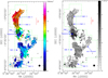 |
Fig. 3 Kinematics of the ISF derived from NH3 (1, 1). Left panel: velocity map (color image) of the ISF. Right panel: FWHM line width map (gray image) of the ISF. Contours in each panel are the same as in the left panel of Fig. 1. The gray solid polyline in the left panel indicates the loci for the position-velocity diagram presented in Fig. 5. |
4.2. Kinematics from NH3
Figure 3 presents the kinematics of the ISF derived from NH3 (1, 1). The left panel displays velocity (color image) and the right panel indicates the intrinsic line width (i.e., for an individual hyperfine component, gray image). They are all derived by the NH3 (1, 1) fitting method in GILDAS. The two images are overlaid with NH3 (1, 1) integrated intensity contours as in Fig. 1. Firstly, we can see that a clear velocity gradient runs along the main part of the ISF. Following the procedure outlined in Goodman et al. (1993), we fitted the velocity gradient as a simple linear form: VLSR = ν0+a× δα +b× δβ, where δα and δβ are offsets in right ascension and declination (in radians), and ν0 presents the systemic velocity of the cloud. The velocity gradient is therefore given by ∇ν = (a2 + b2)0.5/D at a distance of D. The derived gradient is 0.6 ± 0.08 km s−1 pc−1 at 414 pc using all the spectra with peak line flux larger than 5σ. This linear velocity fitting is based on a solid body approximation for the ISF. To check this assumption, we study the velocity residuals (Vobs–Vrigid) in Appendix D. The velocity residuals do not present major departures from a linear velocity distribution. The observed velocity gradient is comparable to the overall rotation of the Orion A Molecular Cloud (e.g., Wilson et al. 2005). Wilson et al. (2005) suggested an increase in the inclination of the filament as a function of time with respect to the line of sight (see Sect. 4.1). Taking the ISF as a homogeneous rigidly rotating cylinder, the ratio of rotational (around its center near δ ∼ −5°30′) to gravitational energy is
where G is the gravitational constant and ρ, L, R, and ω are the density, height, radius and the angular velocity of the cylinder. x ≡ L/D, f(x) ∼ 1 (Bonnell et al. 1992).
We can also write this as
where, ω−14 is the angular velocity in units of 10−14 s−1 and n4 is the gas density in units of 104 cm−3 (Menten et al. 1984; Levshakov et al. 2013). Adopting an angular velocity of 1.94 × 10⁻¹⁴ s−1 and an average density of the ISF of 104 cm−3 (Bally et al. 1987; Dutrey et al. 1991; Berné et al. 2014), then β ∼ 0.25. Thus, the rotational energy is a small fraction of the gravitational energy.
From the line width image, three patterns are apparent. Firstly, the most dispersed region is located around the Trapezium in OMC-1. Secondly, in the northern part of the ISF, very low and also uniform intrinsic (for individual hyperfine components) dispersions (σ ∼ 0.4 ± 0.08 km s−1) are present. Very narrow line widths of the NH3 (1, 1) main line are mostly found in this region. Thirdly, irregular and larger dispersion is present in the southern part of the ISF. This may mainly be because in this region S/Ns are not as high. We study the FWHM line widths of the NH3 (1, 1) main lines with a peak line flux threshold of 5σ as summarized in Fig. 4. The line width refers to individual hyperfine component and is fitted using the GILDAS built-in “NH3 (1, 1)” fitting method. Obviously the line width distribution of the NH3 (1, 1) gas has an outstanding peak around 1 km s−1 Therefore we adopted this line width as the typical width for the fragmentation analysis in Sect. 4.1. The median and mean intrinsic line widths are 1.3 km s−1 and 1.5 km s−1, respectively.
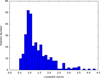 |
Fig. 4 Histograms of the intrinsic FWHM line widths of the NH3 (1, 1) main lines. These line widths referring to individual hyperfine components are derived from the GILDAS built-in “NH3 (1, 1)” fitting which can fit all 18 hyperfine components simultaneously. |
To clearly show the kinematics along the ISF, we created the poly-line position-velocity (PV) diagram presented in Fig. 5. The loci of the PV diagram, which runs through the ridge of the ISF and crosses the cores, are illustrated by the gray solid lines in the left panel of Fig. 3. We averaged 5 pixels (5′) perpendicular to the loci in order to present the integral kinematics and to make sure that the exact location of the poly-line, chosen by eye, is not a critical parameter. From the diagram, we can see that, (1) there is an overall velocity gradient along the ISF as shown in the velocity image (left panel of Fig. 3); (2) bounded by OMC-1, the features of the northern part are coherent and compact, and the southern ones are diffuse and faint; and (3) the two sub-clumps in the OMC-1 show a large difference in velocity.
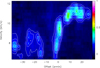 |
Fig. 5 Position-velocity (PV) diagram of the NH3 (1, 1) main line along the gray solid poly-line in the left panel of Fig. 3. The cut runs through the ISF with negative offsets referring to the southern part of the filament. Offset 0 refers to the location of the Trapezium cluster. The threshold and step of the contours of the position-velocity diagram are all 10% of the peak flux. |
Filamentary structures of MCs may be seen as accretion channels to their associated clumps and lead to a seesaw velocity distribution (e.g., Kirk et al. 2013; Zhang et al. 2015). Therefore, to further examine the gas kinematics, Fig. 6 presents the centroid velocity obtained by the main lines of NH3 (1, 1). We firstly excluded the spectra with peak line flux less than 5σ to avoid spurious results. We then averaged the spectra within a 1′-wide belt in declination along right ascension which is roughly perpendicular to the main filamentary structure. Finally, single Gaussian fits were used to get the centroid velocities of these averaged spectra. The result is summarized in Fig. 6 with blue dots and lines. Beside the overall motion (velocity gradient), fluctuations are also seen along the ISF. The locations of OMC-1 to 5 are labeled in this figure and are all found near the local extrema of the fluctuations. This may hint at gas flows toward the clumps in the ISF but may also arise from effects related to star formation. Besides, we also derive the centroid velocities of IRAM 13CO (2-1) data with the same method as for NH3 and summarize this in Fig. 6 with red dots and lines. The large velocity shifts and fluctuations are roughly the same as for NH3. However, there is a striking velocity jump (∼2 km s−1) of NH3 relative to 13CO around OMC-1. According to 13CO observations in Orion A (e.g., Bally et al. 1987; Berné et al. 2014), the northern part of the Orion A molecular cloud is a coherent structure. It is not likely that 13CO is from a separate group of clouds along the line of sight. Considering the strong NH3 emission originating from OMC-1’s dense hot core with a radial velocity of ∼5 km s−1, while that of the nearby Orion ridge, which dominates the 13CO emission, is near 8 km s−1 (e.g., Genzel et al. 1982; Wiseman & Ho 1998), the discrepancy is readily explained.
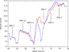 |
Fig. 6 The centroid velocities of the NH3 (1, 1) (blue dots and lines) and 13CO(1-0) (red dots and lines) averaged in 1′-width belts in declination along the ISF. Offset 0 refers to the location of the Trapezium cluster. The locations of OMC-1 to 5 are also displayed in this panel. |
4.3. Temperature
The lack of allowed radiative transitions between the K = 1 and 2 ladders of NH3 makes their relative populations highly sensitive to collisions, therefore making them a good estimator of the gas kinetic temperature. The rotation temperature of the two levels is derived following the method in Ho & Townes (1983). The integrated optical depth of the main feature of the NH3 (1, 1) transition, excluding the satellite lines, is derived by the GILDAS built-in “NH3 (1, 1)” fitting method. Subsequently, we used the formula below to obtain the rotational temperature,
![$$ T_\mathrm{rot}{(2,2\;:1,1)}=-41.5\div\ln\left[\frac{-0.282}{\tau_\mathrm m{(1,1)}}\ln\left[1-\frac{\mathrm\Delta T_\mathrm a{(2,2,m)}}{\mathrm\Delta T_\mathrm a{(1,1,m)}}\right]{(1-\exp^{-\tau_\mathrm m{(1,1)}})}\right], $$](/articles/aa/full_html/2018/08/aa30316-16/aa30316-16-eq8.gif)
where ΔT is the main line intensity and τm denotes the main group opacity derived using the GILDAS built-in ‘NH3 (1, 1)’ fitting. ΔT of NH3 (1, 1) and NH3 (2, 2) are derived using the GILDAS built-in ‘GAUSS’ fitting. The mean uncertainty of the derived temperature is 2 K.
The color image in the left panel of Fig. 7 presents the rotational temperature (TR) distribution of the ISF with overlaid NH3 (1, 1) integrated intensity contours as in Fig. 1. TR exceeds 40 K towards several positions. There the intensities of NH3 (2, 2) are even stronger than those of NH3 (1, 1) and they mainly come from OMC-1. As an example, nine spectra around the Trapezium are presented in the right-bottom panel of Fig. 7 (black spectra for NH3 (1, 1), red spectra for NH3 (2, 2)). From the left panel we can see, the gas around the Trapezium cluster is characterized by TR ∼ 30–40 K. The gas in OMC-2, OMC-3, and the northern part of OMC-4 has a lower TR of about 20 K or even lower than that. In OMC-2 to 4, we can see higher TR at the boundaries and lower TR in the interior of these clumps. This may illustrate that heating originates mainly from the outside and that these clumps may still be in an early evolutionary stage.
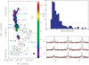 |
Fig. 7 Left panel: temperature distribution along the ISF overlaid with integrated intensity contours as in the left panel of Fig. 1. Most of the temperatures are about or below 20 K. Temperatures exceed 40 K at several positions. There the NH3 (2, 2) lines are even stronger than those of NH3 (1, 1) (see the lower right panel). Top right panel: histogram of the rotation temperatures derived from NH3. Lower right panel: the NH3 (1, 1) (black profiles) and NH3 (2, 2) (red profiles) spectra around the Trapezium. The reference position corresponds to RA: 05:35:14, DEC: −05:22:24(J2000), the spacing is one arcminute. |
A statistical distribution of TR is summarized in the top-right panel of Fig. 7 and shows a typical value of about 16 K, corresponding to a kinetic temperature of 18 K (following Tafalla et al. 2004), which has been used in Sect. 4.1 to calculate expected clump separations inside a cloud of cylindric morphology. The median and mean values are 19 K and 20.8 K, corresponding to a kinetic temperature of 23 K and 26 K (following Tafalla et al. 2004).
4.4. A brief comparison with GBT data
While this work was in progress, Friesen et al. (2017) published ammonia data of the ISF obtained with the Green Bank Telescope. This map, taken with a resolution of 32″, extends slightly further to the south but is limited to the narrow ridge and does not include the western protrusion of the filament we see between δ ∼ −5°25′ and δ ∼ −5°40′. Agreement in the overall velocity, line width, and kinetic temperature distributions is fairly good. We also identify the cloud displaced 5′–10′ eastwards of the backbone of the filament near δ ∼ −5°52′.
5. Summary
We have mapped the ISF in NH3 (1, 1) and (2, 2) located at the northern end of the Orion A molecular cloud. The uniformly and fully-sampled observations cover a region of about 1.2 degrees in declination and about 0.6 degrees in right ascension. The main conclusions of this work are as follows.
The NH3 morphology of the ISF is associated with the Herschel infrared dust ridge and also shows an ISF morphology. A 2-pc-length “sub-filament” extruding toward the northwest of OMC-4 also shows a clear corresponding far infrared feature and is detected for the first time in NH3.
We identify 6 clumps and 11 sub-clumps in the integrated intensity maps of NH3 (1, 1). We find the clumps and sub-clumps are all separated not randomly but in roughly equal intervals. Comparing our data with (quasi-) periodically spaced fragmentation in the ISF revealed by previous studies, we propose that hierarchical fragmentation around the clump scale (∼1 pc) shows two levels, that is, clumps at separations of 1.36 ± 0.16 pc and sub-clumps with a spacing of 0.86 ± 0.14 pc. Adopting an inclination of 60°, this two-level fragmentation is consistent with turbulent and thermal fragmentation inside a gas cloud with cylindric morphology.
A velocity gradient of 0.6 km s−1 pc−1 runs along the ISF, likely due to an overall rotation of the Orion A cloud. Using this velocity, we compared rotational and gravitational energy of the ISF. The ratio is about 0.25, demonstrating that the rotational energy is a small fraction of the gravitational energy. We made an averaged centroid velocity diagram along the ISF to check the roles of filaments as the accretion channels to clumps. From the diagram, fluctuations are seen along the ISF. OMC-1 to 5 are all located near local extrema of the fluctuations. This may indicate gas flows toward the clumps in the ISF but may also be explained in terms of star forming activity. Moreover, a striking velocity jump of NH3 relative to 13CO around the OMC-1 is found in this diagram. The explanation is that NH3 is enhanced by hot dense clumps while 13CO is mainly associated with less dense cooler gas.
The derived NH3 (1, 1) and (2, 2) rotation temperatures in the OMC-1 are about 30–40 K. Lower rotation temperatures (below 20 K) are present at the northern and the southern parts of the ISF. OMC-2, OMC-3, and northern part of OMC-4 show larger temperatures at the boundaries and lower temperatures in the interior of these clumps. This may illustrate that heating mainly occurs from the outside and that these clumps may still reside in an early evolutionary stage.
This research made use of Montage. It is funded by the National Science Foundation under Grant Number ACI-1440620, and was previously funded by the National Aeronautics and Space Administration’s Earth Science Technology Office, Computation Technologies Project, under Cooperative Agreement Number NCC5-626 between NASA and the California Institute of Technology.
Acknowledgments
This work was funded by the Program of the Light in China’s Western Region (LCRW) under grant Nos. and 2015-XBQN-B-03 and the National Nature Science foundation of China under grant 11433008, 11603063, partly supported by the National Natural Science foundation of China under grant 11373062, 11303081. K.Q. acknowledges the support from National Natural Science Foundation of China (NSFC) through grants NSFC 11473011 and NSFC 11590781.
Appendix A
Calibration stability
The system temperature was calibrated against a signal injected by a noise diode, whose temperature is commonly determined by hot (ambient temperature) and cold (liquid nitrogen) loads. Because of a hardware problem, the output power of the diode noise source was abnormal but could maintain a constant value during the observations. To check the calibration stability, we observed the reference position (with (0, 0) offset) every 2–3 h. The spectral line fluxes turned out to be stable but no absolute flux calibration could be obtained from the data themselves. All observations of the reference position were made in the OTF mode of a small area of 3′×3′. We regridded the data and then fitted the NH3 (1, 1) main lines (the central group of NH3 (1, 1) hyperfine components) to present the peak intensity distribution against elevation (Fig. A.1). We can see in Fig. A.1 that there is no significant systematic variation and the dispersion is relatively small. The statistical error of the peak intensities is 9.5%.
 |
Fig. A.1 Uncorrected NH3 (1, 1) main line intensities against elevation of repeated observations toward the reference position. The position corresponds to RA: 05:35:14, Dec: −05:22:24 (J2000). The statistical error of the flux is about 9.5%. The dotted line indicates a linear fit. |
In order to calibrate our data to the main beam brightness temperature (Tmb) scale, we conducted a comparative analysis between the GBT (Friesen et al. 2017) and our NH3 (1, 1) spectra. The GBT data were calibrated to Tmb scale with an estimated calibration uncertainty of about 10% (Friesen et al. 2017). We smoothed the GBT data to our beamsize using the “XY_MAP” routine in GILDAS. For the process our spectral cube was used as a template. We fitted the NH3 (1, 1) main lines of the reference position and the derived peak line intensities are 2.46 K and 0.46 K for the GBT and our spectra respectively. Therefore our NH3 data were all multiplied by the factor of 2.46/0.46 ≈ 5.31. The GBT spectrum (black) and our spectrum (red, multiplied by 5.31) of the reference position are illustrated in Fig. A.2. We estimate our calibration uncertainty to be 
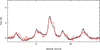 |
Fig. A.2 The NH3 (1, 1) spectra from the GBT (black) and our data (red, multiplied by 5.31) toward the reference position RA: 05:35:14, Dec: −05:22:24 (J2000). |
Appendix B
The sub-structures identified by the clumpfind algorithm
To more clearly present the sub-structures identified by the clumpfind algorithm, we colorized the pixels used to define the sub-structures in Fig. B.1. We can see these sub-structures are all related to the emission peaks and are composed of a considerable number of pixels. We should note that there are three sub-structures identified in OMC-4. The separation of the lower two sub-structures in OMC-4 may not be quite that obvious. There is indeed an emission peak at the center of OMC-4 beside the northern and southern ones.
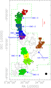 |
Fig. B.1 The colorized pixels illustrate the areas of the 11 sub-structures identified by the clumpfind algorithm. Contours are the same as in the left panel of Fig. 1. Yellow filled circles are same as in the right panel of Fig. 2. |
Appendix C
Dissipation of turbulent energy
Since the clump OMC-2 exhibits lower temperature and simpler structure (OMC-2 has only one sub-clump) than the other clumps, we used this relatively quiescent clump to roughly estimate the velocity dispersion at different scales. We averaged the spectra within squared regions with side lengths of 11′, 9′, 7′, 5′, and 3′ respectively which are all centered at the red cross in OMC-2 illustrated in the right panel of Fig. 2 (see the images in Fig. C.1). We fitted the averaged spectrum using the GILDAS built-in “NH3 (1, 1)” fitting method (see the spectra in Fig. C.1). The derived intrinsic line widths referring to individual hyperfine components, ΔVobs, are 1.22 ± 0.062 km s−1, 1.11 ± 0.046 km s−1, 1.03 ± 0.032 km s−1, 0.94 ± 0.022 km s−1, and 0.88 ± 0.017 km s−1 respectively. All the results above are summarized in Table C.1. The results are also displayed in Fig. C.2 in the form of σV/σT versus side length, where, σT is the thermal velocity dispersion, which is commonly expressed in units of the the sound speed as  . The mean temperature of OMC-2 derived from the averaged spectra of NH3 (1, 1) and (2, 2) is about 20 K. We can see that as the size length decreases, the velocity dispersion decreases and this decrease is approximately linear. Thus, the turbulence dissipates in the inner part of the ISF and we speculate that the thermal pressure of gas becomes more dominant.
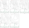 |
Fig. C.1. From left to right and top to bottom, the contours are the integrated intensity (zeroth moment) maps of NH3 (1, 1) with side lengths of 11′, 9′, 7′, 5′, and 3′ respectively. These images are all centered at the red cross in OMC-2 illustrated in the right panel of Fig. 2. The integration range of each panel is 6.5 < VLSR < 12.5 km s−1. Contours start at 0.96 K km s−1 (4σ) and go up in steps of 0.96 K km s−1. The spectra (black) overlaid with their fitting curves (green) are the averaged spectra within the regions corresponding to their upper panels. |
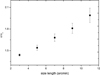 |
Fig. C.2 The ratio of observed to thermal velocity dispersion, σV/σT, derived from the averaged spectra in Fig. C.1 against the side length of the averaged regions. |
We can see that in Fig. C.1, absorption features are present at 6 km s−1 and 20 km s−1. In fact, the right side of the main line and all satellite lines present potential absorption features. However, the main line with broader line width covers the absorption feature. By checking the raw data, these features are not from emission by the reference position. However, the S/Ns of these features are all lower than 1.8 and they are therefore not analyzed in this work.
Appendix D
The residuals of the velocity fitting
The linear velocity fitting is based on the assumption that the ISF is a rigid body. To check this assumption, we present the distribution of the velocity residuals between the observed velocity and the fitting velocity in Fig. D.1 and also the statistics of the velocity residuals in Fig. D.2. From Fig. D.1, we can see that most of the velocity residuals are distributed in the range Vobs–Vrigid = −1 km s−1 to 1 km s−1 which is even more clearly presented in Fig. D.2. The larger velocity residuals are mainly negative and mostly located at the southern part of OMC-1 and the northern part of OMC-4. In general, the velocity residuals do not present major departures from a linear velocity distribution.
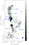 |
Fig. D.1 Velocity residual (Vobs–Vrigid) map (gray image) of the ISF derived from our NH3. Contours are as in the left panel of Fig. 1. |
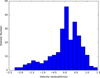 |
Fig. D.2 Histograms of the velocity residuals (Vobs–Vrigid) derived from our NH3. |
References
- André, P., Men’shchikov, A., Bontemps, S., et al. 2010, A&A, 518, L102 [NASA ADS] [CrossRef] [EDP Sciences] [Google Scholar]
- André, P., Di Francesco, J., Ward-Thompson, D., et al. 2014, Protostars and Planets VI, 27 [Google Scholar]
- Bally, J. 2008, in Overview of the Orion Complex, ed. B. Reipurth, 459 [Google Scholar]
- Bally, J., Langer, W. D., Stark, A. A., & Wilson, R. W. 1987, ApJ, 312, L45 [NASA ADS] [CrossRef] [Google Scholar]
- Barranco, J. A., & Goodman, A. A. 1998, ApJ, 504, 207 [NASA ADS] [CrossRef] [Google Scholar]
- Berné, O., Marcelino, N., & Cernicharo, J. 2014, ApJ, 795, 13 [NASA ADS] [CrossRef] [Google Scholar]
- Bonnell, I., Arcoragi, J.-P., Martel, H., & Bastien, P. 1992, ApJ, 400, 579 [NASA ADS] [CrossRef] [Google Scholar]
- Cesaroni, R., & Wilson, T. L. 1994, A&A, 281, 209 [NASA ADS] [Google Scholar]
- Chandrasekhar, S., & Fermi, E. 1953, ApJ, 118, 116 [NASA ADS] [CrossRef] [MathSciNet] [Google Scholar]
- Danby, G., Flower, D. R., Valiron, P., Schilke, P., & Walmsley, C. M. 1988, MNRAS, 235, 229 [NASA ADS] [CrossRef] [Google Scholar]
- Dutrey, A., Duvert, G., Castets, A., et al. 1991, A&A, 247, L9 [Google Scholar]
- Evans, II, N. J. 1999, ARA&A, 37, 311 [NASA ADS] [CrossRef] [Google Scholar]
- Friesen, R. K., Pineda, J. E., co-PIs, et al. 2017, ApJ, 843, 63 [NASA ADS] [CrossRef] [Google Scholar]
- Genzel, R., & Stutzki, J. 1989, ARA&A, 27, 41 [NASA ADS] [CrossRef] [Google Scholar]
- Genzel, R., Ho, P. T. P., Bieging, J., & Downes, D. 1982, ApJ, 259, L103 [NASA ADS] [CrossRef] [Google Scholar]
- Goodman, A. A., Benson, P. J., Fuller, G. A., & Myers, P. C. 1993, ApJ, 406, 528 [NASA ADS] [CrossRef] [Google Scholar]
- Goodman, A. A., Barranco, J. A., Wilner, D. J., & Heyer, M. H. 1998, ApJ, 504, 223 [NASA ADS] [CrossRef] [Google Scholar]
- Hanawa, T., Nakamura, F., Matsumoto, T., et al. 1993, ApJ, 404, L83 [NASA ADS] [CrossRef] [Google Scholar]
- Ho, P. T. P., & Townes, C. H. 1983, ARA&A, 21, 239 [NASA ADS] [CrossRef] [Google Scholar]
- Hunter, J. D. 2007, Comput. Sci. Eng., 9, 90 [Google Scholar]
- Inutsuka, S.-I., & Miyama, S. M. 1992, ApJ, 388, 392 [NASA ADS] [CrossRef] [Google Scholar]
- Jackson, J. M., Finn, S. C., Chambers, E. T., Rathborne, J. M., & Simon, R. 2010, ApJ, 719, L185 [NASA ADS] [CrossRef] [Google Scholar]
- Johnstone, D., & Bally, J. 1999, ApJ, 510, L49 [NASA ADS] [CrossRef] [Google Scholar]
- Johnstone, D., & Bally, J. 2006, ApJ, 653, 383 [Google Scholar]
- Kainulainen, J., Ragan, S. E., Henning, T., & Stutz, A. 2013, A&A, 557, A120 [NASA ADS] [CrossRef] [EDP Sciences] [Google Scholar]
- Kirk, H., Myers, P. C., Bourke, T. L., et al. 2013, ApJ, 766, 115 [NASA ADS] [CrossRef] [Google Scholar]
- Kounkel, M., Hartmann, L., Loinard, L., et al. 2017, ApJ, 834, 142 [NASA ADS] [CrossRef] [Google Scholar]
- Levshakov, S. A., Henkel, C., Reimers, D., et al. 2013, A&A, 553, A58 [NASA ADS] [CrossRef] [EDP Sciences] [Google Scholar]
- Li, D. L., Esimbek, J., Zhou, J. J., et al. 2014, A&A, 567, A10 [NASA ADS] [CrossRef] [EDP Sciences] [Google Scholar]
- Lu, X., Zhang, Q., Liu, H. B., Wang, J., & Gu, Q. 2014, ApJ, 790, 84 [NASA ADS] [CrossRef] [Google Scholar]
- Maddalena, R. J., Morris, M., Moscowitz, J., & Thaddeus, P. 1986, ApJ, 303, 375 [NASA ADS] [CrossRef] [Google Scholar]
- Menten, K. M., Walmsley, C. M., Kruegel, E., & Ungerechts, H. 1984, A&A, 137, 108 [NASA ADS] [Google Scholar]
- Menten, K. M., Reid, M. J., Forbrich, J., & Brunthaler, A. 2007, A&A, 474, 515 [NASA ADS] [CrossRef] [EDP Sciences] [Google Scholar]
- Ohashi, S., Sanhueza, P., Chen, H.-R. V., et al. 2016, ApJ, 833, 209 [NASA ADS] [CrossRef] [Google Scholar]
- Ostriker, J. 1964, ApJ, 140, 1056 [NASA ADS] [CrossRef] [MathSciNet] [Google Scholar]
- Ott, S. 2010, in Astronomical Data Analysis Software and Systems XIX, eds. Y. Mizumoto, K.-I. Morita, & M. Ohishi, ASP Conf. Ser., 434, 139 [NASA ADS] [Google Scholar]
- Pineda, J. E., Rosolowsky, E. W., & Goodman, A. A. 2009, ApJ, 699, L134 [NASA ADS] [CrossRef] [Google Scholar]
- Schneider, S., & Elmegreen, B. G. 1979, ApJS, 41, 87 [NASA ADS] [CrossRef] [Google Scholar]
- Shirley, Y. L. 2015, PASP, 127, 299 [NASA ADS] [CrossRef] [Google Scholar]
- Stutz, A. M., & Kainulainen, J. 2015, A&A, 577, L6 [NASA ADS] [CrossRef] [EDP Sciences] [Google Scholar]
- Tafalla, M., Myers, P. C., Caselli, P., & Walmsley, C. M. 2004, A&A, 416, 191 [NASA ADS] [CrossRef] [EDP Sciences] [Google Scholar]
- Takahashi, S., Ho, P. T. P., Teixeira, P. S., Zapata, L. A., & Su, Y.-N. 2013, ApJ, 763, 57 [NASA ADS] [CrossRef] [Google Scholar]
- Tan, J. C., Beltrán, M. T., Caselli, P., et al. 2014, Protostars and Planets VI, 149 [Google Scholar]
- Teixeira, P. S., Takahashi, S., Zapata, L. A., & Ho, P. T. P. 2016, A&A, 587, A47 [NASA ADS] [CrossRef] [EDP Sciences] [Google Scholar]
- Walmsley, C. M., & Ungerechts, H. 1983, A&A, 122, 164 [NASA ADS] [Google Scholar]
- Wang, K., Zhang, Q., Testi, L., et al. 2014, MNRAS, 439, 3275 [NASA ADS] [CrossRef] [Google Scholar]
- Williams, J. P., de Geus, E. J., & Blitz, L. 1994, ApJ, 428, 693 [NASA ADS] [CrossRef] [Google Scholar]
- Wilson, B. A., Dame, T. M., Masheder, M. R. W., & Thaddeus, P. 2005, A&A, 430, 523 [NASA ADS] [CrossRef] [EDP Sciences] [Google Scholar]
- Wiseman, J. J., & Ho, P. T. P. 1998, ApJ, 502, 676 [NASA ADS] [CrossRef] [Google Scholar]
- Zhang, Q., Wang, Y., Pillai, T., & Rathborne, J. 2009, ApJ, 696, 268 [NASA ADS] [CrossRef] [Google Scholar]
- Zhang, Q., Wang, K., Lu, X., & Jiménez-Serra, I. 2015, ApJ, 804, 141 [NASA ADS] [CrossRef] [Google Scholar]
- Zinnecker, H., & Yorke, H. W. 2007, ARA&A, 45, 481 [NASA ADS] [CrossRef] [Google Scholar]
All Tables
All Figures
|
Fig. 1. Integrated intensity (zeroth moment) maps of NH3 (1, 1) (left) and (2, 2) (right). The integration range of each panel is 6.5 < VLSR < 12.5 km s−1. Contours start at 0.96 K km s−1 (4σ) on a main beam brightness temperature scale and go up in steps of 0.96 K km s−1. The limits of the mapped region are indicated with green dashed lines. A blue star in each panel indicates the Trapezium cluster and black filled circles in the lower right illustrate the half-power beam size. |
| In the text | |
|
Fig. 2 Left panel: false color image of the ISF (red for 500 μm, green for 250 μm, and blue for 100 μm, all Herschel data) overlaid with NH3 (1, 1) integrated intensity contours, as in Fig. 1. Right panel: “clumps” and “sub-clumps” are labeled as red crosses and yellow filled circles, respectively, on the NH3 (1, 1) integrated intensity map. |
| In the text | |
|
Fig. 3 Kinematics of the ISF derived from NH3 (1, 1). Left panel: velocity map (color image) of the ISF. Right panel: FWHM line width map (gray image) of the ISF. Contours in each panel are the same as in the left panel of Fig. 1. The gray solid polyline in the left panel indicates the loci for the position-velocity diagram presented in Fig. 5. |
| In the text | |
|
Fig. 4 Histograms of the intrinsic FWHM line widths of the NH3 (1, 1) main lines. These line widths referring to individual hyperfine components are derived from the GILDAS built-in “NH3 (1, 1)” fitting which can fit all 18 hyperfine components simultaneously. |
| In the text | |
|
Fig. 5 Position-velocity (PV) diagram of the NH3 (1, 1) main line along the gray solid poly-line in the left panel of Fig. 3. The cut runs through the ISF with negative offsets referring to the southern part of the filament. Offset 0 refers to the location of the Trapezium cluster. The threshold and step of the contours of the position-velocity diagram are all 10% of the peak flux. |
| In the text | |
|
Fig. 6 The centroid velocities of the NH3 (1, 1) (blue dots and lines) and 13CO(1-0) (red dots and lines) averaged in 1′-width belts in declination along the ISF. Offset 0 refers to the location of the Trapezium cluster. The locations of OMC-1 to 5 are also displayed in this panel. |
| In the text | |
|
Fig. 7 Left panel: temperature distribution along the ISF overlaid with integrated intensity contours as in the left panel of Fig. 1. Most of the temperatures are about or below 20 K. Temperatures exceed 40 K at several positions. There the NH3 (2, 2) lines are even stronger than those of NH3 (1, 1) (see the lower right panel). Top right panel: histogram of the rotation temperatures derived from NH3. Lower right panel: the NH3 (1, 1) (black profiles) and NH3 (2, 2) (red profiles) spectra around the Trapezium. The reference position corresponds to RA: 05:35:14, DEC: −05:22:24(J2000), the spacing is one arcminute. |
| In the text | |
|
Fig. A.1 Uncorrected NH3 (1, 1) main line intensities against elevation of repeated observations toward the reference position. The position corresponds to RA: 05:35:14, Dec: −05:22:24 (J2000). The statistical error of the flux is about 9.5%. The dotted line indicates a linear fit. |
| In the text | |
|
Fig. A.2 The NH3 (1, 1) spectra from the GBT (black) and our data (red, multiplied by 5.31) toward the reference position RA: 05:35:14, Dec: −05:22:24 (J2000). |
| In the text | |
|
Fig. B.1 The colorized pixels illustrate the areas of the 11 sub-structures identified by the clumpfind algorithm. Contours are the same as in the left panel of Fig. 1. Yellow filled circles are same as in the right panel of Fig. 2. |
| In the text | |
|
Fig. C.1. From left to right and top to bottom, the contours are the integrated intensity (zeroth moment) maps of NH3 (1, 1) with side lengths of 11′, 9′, 7′, 5′, and 3′ respectively. These images are all centered at the red cross in OMC-2 illustrated in the right panel of Fig. 2. The integration range of each panel is 6.5 < VLSR < 12.5 km s−1. Contours start at 0.96 K km s−1 (4σ) and go up in steps of 0.96 K km s−1. The spectra (black) overlaid with their fitting curves (green) are the averaged spectra within the regions corresponding to their upper panels. |
| In the text | |
|
Fig. C.2 The ratio of observed to thermal velocity dispersion, σV/σT, derived from the averaged spectra in Fig. C.1 against the side length of the averaged regions. |
| In the text | |
|
Fig. D.1 Velocity residual (Vobs–Vrigid) map (gray image) of the ISF derived from our NH3. Contours are as in the left panel of Fig. 1. |
| In the text | |
|
Fig. D.2 Histograms of the velocity residuals (Vobs–Vrigid) derived from our NH3. |
| In the text | |
Current usage metrics show cumulative count of Article Views (full-text article views including HTML views, PDF and ePub downloads, according to the available data) and Abstracts Views on Vision4Press platform.
Data correspond to usage on the plateform after 2015. The current usage metrics is available 48-96 hours after online publication and is updated daily on week days.
Initial download of the metrics may take a while.