| Issue |
A&A
Volume 577, May 2015
|
|
|---|---|---|
| Article Number | A85 | |
| Number of page(s) | 14 | |
| Section | Extragalactic astronomy | |
| DOI | https://doi.org/10.1051/0004-6361/201425275 | |
| Published online | 08 May 2015 | |
Extensive light profile fitting of galaxy-scale strong lenses
Towards an automated lens detection method
Institut d’Astrophysique de Paris, UMR7095 CNRS &
Université Pierre et Marie Curie, 98bis Bd Arago, 75014
Paris,
France
e-mail:
brault@iap.fr
Received: 4 November 2014
Accepted: 3 February 2015
Aims. We investigate the merits of a massive forward-modeling of ground-based optical imaging as a diagnostic for the strong lensing nature of early-type galaxies, in the light of which blurred and faint Einstein rings can hide.
Methods. We simulated several thousand mock strong lenses under ground- and space-based conditions as arising from the deflection of an exponential disk by a foreground de Vaucouleurs light profile whose lensing potential is described by a singular isothermal ellipsoid. We then fitted for the lensed light distribution with sl_fit after subtracting the foreground light emission (ideal case) and also after fitting the deflector light with galfit. By setting thresholds in the output parameter space, we can determine the lensed or unlensed status of each system. We finally applied our strategy to a sample of 517 lens candidates in the CFHTLS data to test the consistency of our selection approach.
Results. The efficiency of the fast modeling method at recovering the main lens parameters such as Einstein radius, total magnification, or total lensed flux is quite similar under CFHT and HST conditions when the deflector is perfectly subtracted (only possible in simulations), fostering a sharp distinction between good and poor candidates. Conversely, a substantial fraction of the lensed light is absorbed into the deflector model for a more realistic subtraction, which biases the subsequent fitting of the rings and then disturbs the selection process. We quantify completeness and purity of the lens-finding method in both cases.
Conclusions. This suggests that the main limitation currently resides in the subtraction of the foreground light. Provided further enhancement of the latter, the direct forward-modeling of large numbers of galaxy-galaxy strong lenses thus appears tractable and might constitute a competitive lens finder in the next generation of wide-field imaging surveys.
Key words: gravitational lensing: strong / methods: data analysis / methods: statistical / techniques: miscellaneous / surveys / galaxies: elliptical and lenticular, cD
© ESO, 2015
1. Introduction
Strong gravitational lensing can be used to great effect to measure the mass profiles of early-type galaxies, both in the nearby Universe and at cosmological distances (e.g., Treu & Koopmans 2002a,b, 2004; Rusin et al. 2003; Koopmans et al. 2006; Jiang & Kochanek 2007; Gavazzi et al. 2007; Treu 2010; Auger et al. 2010; Lagattuta et al. 2010; Sonnenfeld et al. 2012; Bolton et al. 2012; Dye et al. 2014; Oguri et al. 2014). Until recently, this approach was severely limited by the small size of the samples of known strong gravitational lenses. With the advent of deep, wide-field imaging surveys we have now entered a new era that enables the use of sizable samples of strong lensing events as precision diagnostics of the physical properties of the distant Universe.
The most abundant configurations of strong lensing events observed to date involve a foreground massive galaxy and a background somewhat fainter source that is well aligned with the former (so-called galaxy-galaxy strong lensing). Even though other recent approaches based on spectroscopic surveys (Bolton et al. 2004, 2006; Auger et al. 2010; Brownstein et al. 2012) or imaging data at submm and mm wavelengths (Negrello et al. 2010; Wardlow et al. 2013; Vieira et al. 2013) have been very successful, there is strong motivation to develop techniques to identify many galaxy-galaxy strong lenses purely in very abundant optical imaging data. Marshall et al. (2005) forecast more than ten such systems per square degree at HST-like depth and resolution. Still, ground-based imaging is a potentially promising avenue thanks to the ready availability of hundreds of square degrees in multiple bands with subarcsecond image quality such as the Canada France Hawaii Legacy Survey (CFHTLS).
This argument motivated the Strong Lensing Legacy Survey (SL2S), which comprised, in addition to a search for group and cluster scale lenses (Einstein radius REin ≳ 3″) (Cabanac et al. 2007; More et al. 2012), a galaxy-scale lens search based on the RingFinder technique (Gavazzi et al. 2014, hereafter G14). The main goal of this latter work was to use newly found lenses at redshift z ~ 0.6 to study the formation and evolution of massive galaxies through a joint strong lensing and stellar-dynamical method (Ruff et al. 2011; Gavazzi et al. 2012; Sonnenfeld et al. 2013a,b, 2014). The main ingredient behind the RingFinder approach of finding galaxy-galaxy strong lenses resides in a simple and fast difference-imaging technique in two bands. Although a fair level of automation and reproducibility was reached by RingFinder, it would be a step forward to gain further insight into the lensing nature of a lens candidate to achieve purer samples: this would indeed reduce the human intervention currently needed to visually classify the systems, as well as the follow-up operations that might become quite expensive for the very large surveys to come.
To this end, we propose a new lens finder that would encode the lens equation through massive modeling of all candidates. So far, fine lens models were performed after the selection process as a way to (in)validate the lens nature of the candidates and give accurate estimates of the lens parameters, if appropriate. In the case of this new finder, it would consist of implementing a fast modeling mode that would precede the decision phase on the candidates status, thus requiring to reach a compromise between speed and robustness. Other improvements can be made at the level of the deflector light subtraction (see, e.g., Joseph et al. 2014) that might relax the RingFinder requirement of two bands and make the selection more complete regarding lenses whose source is not blue. Therefore, a promising strategy would be to quickly fit to single-band imaging data a lens model featuring a simple background source and a simple foreground deflector with a small number of degrees of freedom. Some ingredients of such a method have been implemented by Marshall et al. (2009) on archival HST data as part of the HAGGLES effort (see also Newton et al. 2009). The assumption of surface brightness conservation made in HAGGLES is sensible for HST images and allows for fast modeling shortcuts. This is not possible, however, for ground-based imaging with seeing of a size similar to the size of lensed features. Therefore the convolution has to be fully implemented by a large point spread function (PSF), and the light coming from the foreground object and that of the background lensed source have to be carefully separated before any attempt to quickly and robustly model the observed light distribution.
In this paper we attempt to implement a versatile lens modeling code, sl_fit (Gavazzi et al. 2007, 2008, 2011, 2012), in a pipeline that will rapidly fit the light distribution around lens candidates with a simple lens model featuring a foreground early-type galaxy (ETG), a background source, and a singular isothermal ellipsoid (SIE) mass distribution. We first used simulated data to test the speed and reliability of our model optimization techniques to finally adjust the compromise between a fast agressive modeling and a good exploration of the parameter space. The ingredients entering the simulations and the modeling assumptions are presented in Sect. 2, while we report on the precision and speed in the recovery of key model parameters in Sect. 3. The next step is to find a set of quantities provided by the output best-fit model that will optimally allow separating the population of simulated lenses from the population of simulated non-lenses. This is the object of Sect. 4. Finally, in Sect. 5, we perform the same modeling approach on the homogeneous sample of SL2S lenses (G14) enriched with additional preselected systems that are also found in the CFHTLS data to determine by how much we can improve the existing selection, both in terms of completeness and purity. We summarize our main results and present our conclusions in Sect. 6.
2. Simulating and modeling strong lenses
2.1. Physical assumptions
For the simulations as well as for the subsequent modeling part, we make the same assumptions as were made in the simulations of G14. We briefly recapitulate the features that are relevant for this work.
The systems involve a foreground deflector whose light distribution is described by an elliptical de Vaucouleurs profile, which reads ![\begin{equation} I(r) = I_0 \exp\left[ -k_4 \left(\frac{r}{\Reff}\right)^{1/4} \right], \end{equation}](/articles/aa/full_html/2015/05/aa25275-14/aa25275-14-eq3.png) (1)with k4 ≃ 7.669 and Reff is the effective or half-light radius and I0 the central surface brightness. To capture elliptical symmetry, we also need to introduce an axial ratio q and a position angle φ. The deflector will always be centered at the origin of the coordinate system.
(1)with k4 ≃ 7.669 and Reff is the effective or half-light radius and I0 the central surface brightness. To capture elliptical symmetry, we also need to introduce an axial ratio q and a position angle φ. The deflector will always be centered at the origin of the coordinate system.
The total mass profile attached to the deflector is described by a singular isothermal ellipsoid. In the simulation, the ellipticity and orientation of the light and mass match, although this is partly relaxed in the modeling (see below). The strength of the mass distribution, that is, its Einstein radius, is given by the velocity dispersion of the isothermal sphere,  where Dls/Ds is the ratio of angular distance between the lens and the source and between the observer and the source. The luminous content and the mass are tightly coupled by scaling relations in the simulation, as described in G14.
A background source with an elliptical exponential light distribution is also placed behind the deflector. The population of lenses and sources are taken from the CFHT-LS catalog of i< 22 early-type galaxies and the COSMOS catalog of faint i< 25 objects, respectively (Capak et al. 2007; Ilbert et al. 2009). Hence, the complex covariance of magnitude, effective radius, and redshifts is naturally captured by these real catalogs.
The simulations and model fitting were consistently performed with sl_mock and sl_fit, which were introduced in G14 and Gavazzi et al. (2007, 2011, 2012), respectively. These two codes share the same image rendering and lensing engines.
2.2. Observational conditions and preparation of the data
To quantify how well lens model parameters can be recovered, we required that our simulated lenses mimic two typical observing conditions for a given input light distribution. We thus focused on a ground-based survey of depth and image quality given to the CFHT-LS Wide (cf. Sect. 5.1). Seeing conditions and exposure times were randomly taken from real CFHTLS conditions. A library of 50 PSF models spanning a broad realistic range of seeing conditions for this survey was built. The input PSFs were directly inferred by subpixel centering of the stars in the CFHTLS data. These PSF images were constructed at the natural  Megacam pixel scale. We simulated observations in the three g,r,i optical channels of CFHT Megacam, and mock deflectors were produced down to a magnitude i ≲ 22. A noise model that captured the contributions of the photon noise of sky and the objects along with readout noise was applied and stored in variance maps. Hence the noise is non-stationary but is very well described by Gaussian statistics of zero mean and dispersion σij for a given pixel ij.
In addition to these ground-based observing conditions, we simulated the same objects under space-based observations as were obtained with the WFPC2 camera and the F606W filter of the HST during the follow-up campaign of SL2S lenses (Gavazzi et al. 2012; Sonnenfeld et al. 2013a). HST observations are 1400 s long and resemble the planned Euclid depth with a slightly redder filter and slightly broader PSF (Laureijs et al. 2012). In that case, images were sampled at a  pixel scale. We used PSF images calculated with TinyTim (Krist et al. 2011). Oversampling by a factor 4 was used in the HST simulations, and the TinyTim PSF were sampled accordingly. To save computing time in the modeling phase, however, we did not refine the sampling of the light distribution predicted by a given model. We verified that this agressive image-rendering does not lead to significant modeling errors. Unless otherwise stated, we therefore did not apply the same ×4 oversampling to the model and the PSF.
The mock observations thus consist of three (CFHT) and one (WFPC2) noisy input images, along with 3+1 input variance map images, and 3+1 input PSF images. Simulated postage stamps are  on a side, but we focused on a smaller fitting window that is
  wide for the subsequent modeling phase. For illustration, we show in Fig. 1 a few simulated systems under the ground and space conditions.
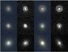 |
Fig. 1 Mosaic of six simulated gravitational lenses under CFHT (gri-color, left) and HST/WFPC2 (gray-scale, right) conditions. Each panel is |

2.3. Subtraction of foreground deflector
In addition, we focused here on modeling the lensed features that are most of the time well buried into the peak of light emitted by the foreground deflector. It is therefore necessary to subtract it before undertaking a precise modeling of the lensed background emission. Thanks to our simulations, we can quantify the impact of imperfect subtraction on the modeling itself. Of course, the photon noise supplied by deflector emission is already taken into account, but we wished to check whether the modeling and, in the end, the decision diagnostic for a lensed or unlensed nature is affected. Marshall et al. (2007) found that at least for high-resolution imaging, either from adaptive optics or from HST imaging, the Einstein radius is well recovered, but that the less-constrained parameters such as source size or shape can be biased. With our simulations, we wish to verify that this is also true for the fast modeling of ground-based data where it is even more difficult to separate the foreground and background emissions. We therefore considered two kinds of deflector subtraction methods:
-
An ideal reference case in which we have a perfect knowledge of the foreground emission. The latter is therefore trivially subtracted. This leaves us with lensed patterns (arcs, rings) that are only affected by noise of known statistics.
-
We also considered galfit (Peng et al. 2002, 2010) to subtract a de Vaucouleurs light profile by trying to mask out the most prominent lensed features in an automated (hence not perfect) way. For ground-based data, we performed a 4σ clipping of the discrepant pixels to down-weight the effect of the lensed features on the fitting of the foreground emission. Moreover, since we are simulating observations in the three gri channels, we performed a four-step fitting, starting from the reddest i-band image (in which the deflector light dominates, on average). This model of the deflector was then used as a starting point for the fit in the r band, which was then used as a starting point for the fit in the g band. Again, we performed a 4σ clipping of discrepant pixels that makes a 1–0 mask that was then used for another fitting of foreground light emission with galfit in g band. The same masking process was applied when subtracting the deflector from observed CFHTLS candidates in Sect. 5 using four bands (griz). For space-based data, we recall that the simulations are carried out in only one filter. Nonetheless, the particular case of space conditions with a galfit subtraction is treated with a finer sampling of the model and the PSF (see Sect. 2.2) to give a sense of the increased execution time. As explained below, this is the only situation in which the finer × 4 sampling was somewhat needed.
2.4. Bayesian inference
We now develop the methodology that we adopted to fit for the lens modeling parameters with the sl_fit tool in a Bayesian framework.
2.4.1. Definitions
The vector of observations, which is the set of pixel values in a small cutout region around a lens candidate, is d. Pixel values are assumed to be devoid of light coming from the foreground deflector, as discussed above.
The posterior probability distribution of the model parameters θ given the observations d is given by the Bayes theorem: 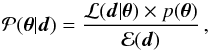 (4)with the usual definition of the likelihood ℒ(d | θ), the prior p(θ), and evidence ℰ(d), which reduces to a normalization constant here since we are testing only a family of models.
The likelihood can be built with the noise properties we have presented above. If we consider an image of size n × n with pixel values stored in a model vector m(θ), we can write ![\begin{equation} \mathcal{L}( \vec{d} \vert \vec{\theta} ) = (2 \pi)^{-n^2/2} \prod_{i=1}^{n^2} \sigma_i^{-1} \exp\left[ -\frac{(d_i-m_i(\vec{\theta}))^2}{2\sigma_i^2}\right] \propto {\rm e}^{-\chi^2/2}. \end{equation}](/articles/aa/full_html/2015/05/aa25275-14/aa25275-14-eq38.png) (5)The assumptions developed in Sect. 2.1 allow predicting the model image m(θ) and specifying the parameters contained in θ. In Table 1, we list them together with the two kinds of priors we assumed for them. For the situation of a galfit subtraction of the deflector, the central values of the priors on the lens potential axis ratio qL and orientation φL are taken from the best-fit value of the galfit optimization. We also used the center of the light profile fitted by galfit as the center of the potential (xc,yc) for the sl_fit modeling, assuming that mass follows light. The case of an ideal subtraction was run later so that we could keep the same values of qL and φL for more consistency between the two subtraction modes; but (xc,yc) are obviously set to (0,0) in this case, as for the simulations.
(5)The assumptions developed in Sect. 2.1 allow predicting the model image m(θ) and specifying the parameters contained in θ. In Table 1, we list them together with the two kinds of priors we assumed for them. For the situation of a galfit subtraction of the deflector, the central values of the priors on the lens potential axis ratio qL and orientation φL are taken from the best-fit value of the galfit optimization. We also used the center of the light profile fitted by galfit as the center of the potential (xc,yc) for the sl_fit modeling, assuming that mass follows light. The case of an ideal subtraction was run later so that we could keep the same values of qL and φL for more consistency between the two subtraction modes; but (xc,yc) are obviously set to (0,0) in this case, as for the simulations.
Definition of model parameters and associated priors.
2.4.2. Optimization scheme
Since we aim to carefully explore the degeneracies in the space of free parameters, we considered a full sampling of the posterior probability distribution with Markov chain Monte Carlo (MCMC) techniques. The practical implementation in sl_fit is the Metropolis-Hastings algorithm. The convergence is accelerated by a burn-in phase (so-called simulated annealing) in which, starting from a pure sampling of the prior, we increasingly give more weight to the likelihood. Defining a pseudo-temperature Tn that decreases with the iteration number n, this reads  (6)After the cooling phase that guides the chain toward the global maximum a posteriori, we can correctly sample the posterior near its maximum. We empirically found that using a total number of iterations Ntot = 2700 was a good compromise between speed and robustness. The last 300 iterations sample the posterior, and the final 100 of them were used for the subsequent statistical analysis of the chain (best-fit parameters and error)1. Hence, our analysis is performed on the most converged part of the chain. In the perspective of massive modeling of many lens candidates, it does not appear very important to have an extremely accurate description of the confidence interval on each model parameter. The MCMC effort remains a robust way to sample complex degeneracies and, for instance, check whether the lensing hypothesis of a given system (that is, the probability that a background source is magnified by more than a certain value is greater than some other value) is consistent with the data.
Despite these benefits, the cost of a full sampling is high in terms of CPU time. Calculations were performed in parallel with modern 2 GHz, 12-core x86_64 servers. As we report below, it takes about 10 s to run a MCMC of length Ntot = 2700 iterations on CFHT g band cutout images.
To reduce the execution time even more in view of a massive modeling sequence for automatic lens detection, we explored the possibility of renouncing the benefits of a Monte Carlo sampling of the posterior PDF and used the faster simplex optimization scheme based on the minuit library2. Gradient methods were also envisioned, but were not reliable enough because of the strong degeneracies between model parameters and multiple local minima, especially for realistic galfit subtractions of the deflector. An option of minuit allows the algorithm to refine its estimate of the parameter covariance matrix at run time and to account for nonsymmetric errors on best-fit parameters. This practicality generally led to many more computationally expensive likelihood estimations, to such a point that it is not competitive with and less robust than our fiducial MCMC method, even in the case of an ideal subtraction. Consequently, we did not retain this fast minimization option in its current implementation in our code because it is not robust enough and produces too many catastrophic failures (especially for a realistic galfit subtraction of the deflector). Nonetheless, the reduced CPU time consumption is a good incentive for improving the parameterization of the problem (to reduce degeneracies), finding better convergence criteria, parallel optimizations, simulated annealing in the minuit phase, etc.
3. Recovery of key lens parameters on mock data
In this section, we assess the recovery by sl_fit of the most relevant quantities that could help deciding whether a foreground galaxy acts as a strong lens on a background source or not. We considered both the CFHTLS-like g band3 and HST WFPC2 simulated images. The most important quantities are the Einstein radius REin, the total magnification μtot, and the total image plane g-band magnitude mimg of the lensed light.
We distinguish the ideal situation of a perfectly subtracted foreground deflector in Sect. 3.1 and the more realistic case of a preliminary subtraction performed with galfit in Sect. 3.2 to show how much the complex crosstalk between foreground and background light (especially for the bright highly magnified sources) has to be treated with caution.
Our deep parent sample of COSMOS sources provides many lensed objects that are too faint to be detectable under CFHTLS conditions or to provide sufficient information for the modeling. Systems with a total magnified flux such that mimg,0> 24.5 are therefore not taken into account in the rest of the analysis.
Figure 5 illustrates the results of such an automated lens-modeling analysis of a simulated ring. Table 2 gathers the main quantitative results. Since we wish to verify that the important lensing parameters are correctly recovered for the most valuable lensing configurations, we mostly considered large magnification systems by restricting the analysis of this section to configurations with a small impact parameter  . The numbers regarding the scatter and bias in the table could change somewhat for large radius less magnified lenses. We checked on a small number of available simulations that the bias is not significantly changed for such systems; obviously, the scatter is slightly increased. Nevertheless, we fully account for this increased dispersion of low-magnification systems in the next section when we exploit sl_fit as a lens-finding tool.
Throughout this article, the subscript 0 refers to input simulation quantities, whereas quantities without this index refer to values actually recovered by sl_fit.
3.1. Comparing ground- and space performance with ideal subtraction of the deflector
Figure 2 shows the difference between recovered and input quantities for the Einstein radius, the image plane total magnitude of the lensed light, and the total magnification.
The Einstein radius is well recovered in the two cases, especially for the highest values, which correspond to complete and bright arcs. We only observe a small bias of about  from the ground-based mock observations for values
  , and
, and  from the space counterparts. This is about a third and a sixth of a pixel, respectively. At smaller radii (
 ), there is more scatter in the recovery of REin for CFHT than for HST mock data: indeed, this population of objects contains an important fraction of faint, low-magnification systems that are poorly resolved from the ground, leaving the model underconstrained.
We also observe a very small bias with a small scatter in the recovery of the total magnified flux of the lensed features, either from ground- or from space-based images. Nevertheless, some outliers appear from HST simulations that did not exist for CFHT simulations: these might be due to the lower resolution of CFHT simulations that leads to a smoother parameter space for the walk of the Markov chain, the convergence of which is made easier. After re-running the modeling procedure on these systems under the same conditions, most of them can be recovered with a value close to the initial one, meaning that the optimization had indeed fallen in a local extremum of the posterior during the first runs, hence illustrating the random character of the MCMC sampling. In the end, these outliers appear negligible, with a rate of a few thousandths.
Despite the good estimation of mimg, there is non-negligible bias in the recovered total magnification μtot from CFHT images for input magnifications above μ0 ~ 2.5, as can be seen in the bottom left panel of Fig. 2. This underestimation bias is not observed for HST simulations. We studied the possible origin of this bias and concluded that it could be due to a slightly too aggressive sampling of the CFHT model when performing a fast modeling. Since mimg is well recovered and mimg = msrc−2.5log 10μtot, this bias is reflected on the recovery of the intrinsic source flux, which is slightly overestimated for CFHT simulations and is good for HST simulations. Here we found μ ~ 0.7μ0, corresponding to msrc ~ msrc,0−0.365.
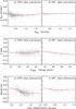 |
Fig. 2 Recovery of Einstein radius (top), total image-plane-lensed flux (middle), and magnification (bottom) for simulated lenses fitted with sl_fit in fast-modeling mode. We distinguish the case of ground-based CFHTLS-Wide-like g-band observations (left) and the case of HST WFPC2/F606W observations (right). In both cases, the deflector light has been “perfectly” subtracted before modeling the residual lensed features. In each panel, the red error bars show the binned median values for guidance. |
Concerning less magnified lensing configurations at large radii, we had a few such simulated systems at our disposal and checked that they mostly add little scatter in the recovery of REin and associated parameters without producing noticeable biases.
For ground-based simulations, the median time for the optimization to complete (i.e., to reach 2700 iterations) is about ~10 s. Only 1% of the chains never converged, and some others took a very long time to complete. We quantified this “failure mode” with the fraction of optimizations that did not converge in less than 1 min. This fraction is about 9% for CFHT simulations. For HST simulations, these numbers rise to a median execution time of ~18 s and a failure rate of ~16% for a threshold value of 2 min. The factor ~2 finer pixel scale of space data explains this increased time. However, we also conclude that our calculations are not yet limited by the rendering of pixels (execution time would scale as  ) but rather by a combination of overheads (disk accesses, MCMC engine, etc.) and a speed-up due to the better defined maximum of the likelihood surface for space data.
3.2. Effect of imperfect galfit subtraction of the deflector
The previous section was optimistically assuming that the light from the foreground deflector could successfully be removed without any implication on the lensed patterns. First of all, any attempt to separate foreground and background emissions is not an easy task for galaxies of a size similar to the seeing disk that emit at similar optical wavelengths. In Sect. 2.3, we proposed a method to mitigate the effect of the background emission when fitting the foreground deflector light with galfit and automated masks.
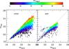 |
Fig. 3 Recovery of the deflector g-band flux when fitted with galfit on CFHT (left) and HST (right) simulations, colored according to the initial magnitude of the lensed light. The lensed background component is oversubtracted in most cases. |
Figure 3 shows the limits of the method. In the left panel, the recovered deflector flux is almost always overestimated for CFHT observations, with a stronger bias for brighter lensed features. This implies that some flux from this latter component has been captured by galfit as belonging to the foreground emission. This reduction of the (large-scale) flux of the arcs is, of course, not desirable and could potentially prevent a lens identification. The right panel concerns HST simulations. The problem is still present, but less pronounced at the faint end; moreover, subtracting the deflector light is clearly less successful for higher values of Δm0 = mimg, 0−mdef,0 (where mdef,0 is the deflector magnitude), especially at the bright end, leaving strong leftover emission in sl_fit input image. We checked that a more careful masking of the lensed features, similar to what can be done one-by-one on a small number of systems (e.g., Bolton et al. 2006; Marshall et al. 2007), alleviates the catastrophic (under-) subtraction of bright deflectors.
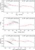 |
Fig. 4 Recovery of Einstein radius (top), total image-plane-lensed flux (middle), and magnification (bottom) for simulated lenses fitted with sl_fit in fast-modeling mode. We distinguish the case of ground-based CFHTLS-wide-like g-band observations (left) and the case of HST WFPC2/F606W observations (right). In both cases, the deflector light has been subtracted with galfit before modeling the residuals. In this case, oversubtracted background emission or undersubtraction or inaccurate modeling of the deflector produces larger errors and biases on fitted important parameters of the lens models. In each panel, the red error bars show the binned median values for guidance. |
The response of modeling the lensed features in the presence of these subtraction defects is complex. The top panels of Fig. 4 show that the Einstein radius is biased in a non-trivial way for ground-based conditions when REin ≲ 1″. This is less the case for space conditions, but still present for  . Obviously, when the lensed features are far away from the deflector, the deflector subtraction tends to the previously discussed case of an ideal subtraction.
At small radii  , the simulated lenses are dominated by double systems with a main arc and a counter-image. From CFHT simulations, the subtraction generally contains little flux because galfit has fitted most of their flux as part of the deflector flux. As a result of this lack of constraints, sl_fit is mainly driven by the priors as it would be for very faint lenses. HST resolution helps identifying the gravitational arcs even when they are faint or very entangled with the deflector: in both cases, galfit absorbs the counter-image, so that the subtraction shows a singly-imaged configuration, leading to an underestimation of the Einstein radius with a characteristic lower bound REin ≲ REin0/2.
At intermediate radii, ( for CFHT,
  for HST), our population of mock lenses already provides a majority of rings or quasi-rings. Concerning CFHT simulations, two net branches show up. For objects where galfit still borrows a big fraction of the lensed flux, the larger Einstein radius causes some part of the arc (not always the brighter part) stand out from the rest of the system, ending up with a singly-imaged lens configuration layout: the Einstein radius is thus underestimated and these lenses make the lower branch of the figure. The upper branch is due to situations in which galfit subtraction leaves a symmetrical residual appear as if an Einstein ring encompassed a hole of negative values. The typical radius is limited by the PSF FWHM IQ. This forces the lens model to predict a ring-like system with REin ≃ max(REin0,IQ) of greater magnification, but with underestimated overall flux (bottom and middle panel). In HST simulations, the resolution at these radii has already distinguished the lensed features from the deflector: the latter is then easily subtracted, taking just little flux from the ring, barely affecting its position or width. Consequently, the lower branch observed from CFHT simulations almost disappears and the upper branch is barely reduced.
Finally, the largest Einstein radii ( for CFHT and,
  for HST) are quite well recovered as the rings are completely separated from the deflector in both HST and CFHT simulations. The few systems in the HST simulations that have large | ΔREin | = | REin − REin0 | are due to the aforementioned failures of the foreground subtraction for some bright objects.
The recovery of the total magnification shows two clearly separated regimes: on one hand, an overestimation regime with a high scatter, on the other hand, a sharp underestimation regime with a small scatter, roughly corresponding to the respective overestimation and underestimation of REin. For HST data, these two modes are significantly alleviated, and for both sets of data, the median value of μ is not highly biased either. The way in which the total flux of the lensed light is recovered somehow echoes the faulty recovery of the deflector flux with galfit: contrary to REin and μ, mimg is thus significantly biased, even for HST data.
We defined the catastrophic errors as the optimizations satisfying | ΔREin | > 10 δREin, the errors being quite underestimated by the fast modeling (see Sect. 2.4.2). With an ideal deflector subtraction, the rate of catastrophic errors is 14% for HST simulations and 38% for CFHT simulations. For a galfit subtraction, this rate remains very similar to its previous value for CFHT simulations, but reaches 41% for HST simulations. We tested that the oversampling of the model-predicted light distribution is needed for HST simulations as it allows the number to catastrophic errors to decrease from 54% to 41%. More precisely, we observe that a low signal-to-noise ratio, low magnification, and low values of REin0 lead to slightly smaller failure fractions (because of the increased formal error δREin), but the dependency of the fraction on either REin0, μ0 or mimg,0 is mild, especially for HST conditions. The dramatic reshuffling of the systems in the recovered parameter space with galfit subtraction washes these trends out.
We now return to less magnified lensing configurations at large radii. Apart from an increased scatter (already mentioned for the case of an ideal deflector subtraction) and a few outliers, our conclusions remain unchanged because multiple image systems still constitute a rather favorable situation for galfit when the Einstein radius is large, the main arc remaining sufficiently far away from the deflector.
Modeling results on the simulated lenses.
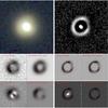 |
Fig. 5 Comparative modeling of a simulated ring in the four cases considered in Sect. 3. Top panels: mock observations of the lens system under CFHT (gri-color, left) and HST/WFPC2 (gray-scale, right) conditions. Other panels: images where the deflector has been subtracted ideally (middle panels) or using galfit (bottom panels), along with the lensed features reconstructed by the model and the critical lines (in red). The CFHT simulations are modeled in the g band. Each panel is |

For ground-based simulations, the median time for the optimization to complete for the subtraction with galfit is similar to the minimization with ideal subtraction, that is ~8 s. However, 14% of the minimizations take more than 1 min to converge, compared to ~9% in the previous case, and among them, more outliers have emerged. This increased failure rate is due to the complex shape of the posterior distribution function often induced by the faulty foreground subtraction. Because of the finer sampling of the light distribution predicted by the model, the median execution time for simulations of space-based data rises to ~6 min. The failure rate reaches 31% for a threshold value of 45 min.
4. Calibrating sl_fit as an automated lens finder with mock data
After we showed that sl_fit accurately estimates the most important parameters that characterize a galaxy-scale strong lensing event, we now proceed with the idea of using the sl_fit output of a given lens model as a way to decide whether it is a gravitational lens or not. All our previous lens modeling assumptions, and in particular the use of galfit to remove the deflector light, were kept unchanged. As already said, we expect that the faulty galfit subtraction will be a source of concern in the lens-finding objective. So we account for this limitation here. From the perspective of using sl_fit as a lens finding algorithm on current and upcoming ground-based datasets, we do not need to discuss the HST simulations in more detail and focus on the CFHT case.
In the previous section, we aimed to assess the reliability of sl_fit at recovering the main lensing parameters that are the Einstein radius, the total magnification μ, and the total magnified flux ming of interesting lenses over a broad range of values regardless of their actual frequency in realistic lensing configurations. To do so, we restricted ourselves to a very small impact parameter for the source  . However, this simulation setup does not reproduce the relative abundance of low- and high-magnification configurations, nor does it uniformly sample the source plane domain over which sl_fit might yield a positive signal. We therefore had to simulate another 3000 systems in the range
  in addition to the already simulated 1260 systems with
  . Hence, the source plane was sampled with two levels of sparsity: a system with a source inside the inner circle was given a statistical weight win = 0.22/2.52 × 3000/1260 ≃ 0.015, while sources inside the outer annulus were given a weight wout = 1−0.22/2.52 ≃ 0.99. In addition to these large impact parameters, low-magnification systems, we also need to account for chance alignment systems that do not give rise to high magnification, but could be flagged by sl_fit output as potential lenses. Systems in which the assumed source actually lies in front of the assumed deflector were therefore included in the statistical analysis of sl_fit output.
To set up the selection, we first classified the simulated lens candidates according to their true characteristics. Following G14, we considered as potentially interesting systems all the previously simulated lines of sight that produced a total magnification μ0> 4 (good lenses), and considered as quite interesting systems with 2 ≤ μ ≤ 4 (average lenses). Moreover, as in the previous section, we did not aim at uncovering lenses for which the magnified arc or ring has a total image plane magnitude mimg,0> 24.5 in the CFHT g band.
We desired our decision process to be simple and therefore designed a binary decision (lens or not-a-lens) based on sl_fit best-fit parameter estimates defined as the median values of the marginal posterior distributions (see Sect. 2.4). Conservative requirements on the quality of the optimization result were also introduced by applying a simple threshold on the reduced χ2/ν statistics. Since the MCMC errors are relatively underestimated by the fast modeling, we did not take them into account.
Figure 6 shows the distribution of the simulated and fitted lens candidates in the {μ, REin, mimg, β} parameter space when the light of the foreground deflector has been ideally subtracted, with a color distinction for “good”, “average” and “non” lenses. Very simple cuts of the kind  (7)are able to isolate the most interesting lenses. We can therefore define the completeness as the number of μ0> 4 systems satisfying definition (7)divided by the total number of μ0> 4 “good” systems. Likewise, we define the purity as the number of μ0> 4 systems satisfying the criterion (7)divided by the total number of systems satisfying the same criterion. We used this simulated sample of lens candidates to maximize the purity as a first step while preserving completeness: Table 3 gathers those results.
Selection results on the simulated lens candidates.
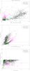 |
Fig. 6 Results of the sl_fit modeling in the {REin, β} (top), {REin, μ} (middle), and {REin, mimg} (bottom) subspaces for an ideal subtraction of the deflector. Three classes of systems are considered: “good lenses” defined by μ0> 4 (pink), “average lenses” such that 2 <μ0< 4 (green), and galaxies that are not lenses (black). Lines represent the empirical cuts applied to isolate lenses. They are defined in Eq. (7). |
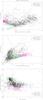 |
Fig. 7 Same as Fig. 6, but for a galfit subtraction of the deflector. Lines represent the cuts defined in Eq. (8). |
In the more realistic case of a galfit subtraction, it is much more difficult to isolate the “good” lenses from galaxies that are not lenses, as can be seen in Fig. 7. The best compromise between completeness and purity is now more difficult to achieve. We came up with the following cuts: 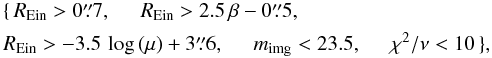 (8)for which the results are also listed in Table 3.
We obtained very good results selecting “good” lenses in the case of an ideal subtraction, ending up with 82% of completeness and 94% of purity. Unfortunately, as a result of the imperfect galfit subtraction spotted in Sect. 3.2 that tends to mix in the parameter space the different areas corresponding to the different classes of lenses, the completeness and purity are substantially reduced to 31% and 69%, respectively. When we individually consider the 2D slices through the involved parameter space, there is a high degree of overlap between the selections resulting from the sets of cuts applied to {REin, β} on the one hand, and to {REin, μ} on the other hand, but we decided to consider both selections here in our attempt to reach a high level of purity. Furthermore, in the case of an ideal subtraction, these two first sets of cuts are at the same time more complete and more selective than the cuts made only through {REin, mimg}. When switching to a galfit subtraction, we find that the selections derived from {REin, β} and {REin, μ} distinguish more precisely than the selection derived from {REin, mimg}, but that the latter is more complete than the second one; furthermore, inside the sample, the selection involving mimg is also more complete for systems with  since, as noted before, galfit systematically assigns a substantial fraction of the lensed flux to the foreground unlensed light distribution when β is small. Average lenses are already quite mixed with unlensed galaxies for an ideally-subtracted deflector, so we did not quantify the completeness and purity relative to that class of lenses. Finally, knowing that we have favored the purity rate, the results remain relatively satisfactory even for the galfit subtraction; but the loss is higher than in the ideal case, which shows that the method chosen for the deflector subtraction plays a crucial role in the lens modeling and the subsequent selection process.
5. Application to real CFHTLS data
We now apply the automated model fitting to the large CFHTLS dataset, whose statistical properties are similar to simulated images. Although we leave a fully automated analysis of the entire survey for a future work, here we make the most of the existing sample of strong lenses built by G14 to test the reliability of our conclusions. We can hence use a large sample of confirmed lenses and good-quality lens candidates to assess the relative completeness between our new method and the previous RingFinder algorithm. In addition, real data add several important new ingredients to the problem that are missing in the simulations, such as a complex morphology of the foreground deflector and background source, but also the environment of potential lenses that is more complex because of neighboring objects that could interfere in the light-fitting process either at the deflector subtraction stage or at the subsequent stage of fitting the residual potentially lensed light.
5.1. SL2S RingFinder sample of strong lenses found in the CFHT-LS
We took advantage of the existing SL2S sample (Ruff et al. 2011; Gavazzi et al. 2012, 2014; Sonnenfeld et al. 2013a,b, 2014) of candidate and confirmed galaxy-scale strong lensing systems found in the CFHTLS with the RingFinder algorithm. The goal was to investigate the response of our automated modeling method to a large number of interesting lens candidates.
The Canada-France-Hawaii Telescope Legacy Survey4 (CFHTLS) is a major photometric survey of more than 450 nights over five years (started on June 1, 2003) using the MegaCam wide-field imager, which covers ~1 square degree on the sky, with a pixel size of 0.̋186. The CFHTLS has two components aimed at extragalactic studies: a Deep component consisting of four pencil-beam fields of 1 deg2 and a Wide component consisting of four mosaics covering 150 deg2 in total. Both surveys are imaged through five broadband filters. In this paper we use the sixth data release (T0006) described in detail by Goranova et al. (2009)5. The Wide survey reaches a typical depth of u∗ ≃ 25.35, g ≃ 25.47, r ≃ 24.83, i ≃ 24.48 and z ≃ 23.60 (AB mag of 80% completeness limit for point sources) with typical FWHM point spread functions of  ,
,  ,
,  ,
,  and
and  , respectively. Because of the greater solid angle, the Wide survey is the most useful component of the CFHTLS for finding and studying strong lenses. Regions around the halo of bright saturated stars, near CCD defects or near the edge of the fields, have lower quality photometry and were discarded from the analysis. Overall, ~21% of the CFHTLS Wide survey area was rejected, which reduced the total usable area to 135.2 deg2.
The RingFinder lens finding method is presented in G14. This algorithm detects compact rings around isolated galaxies and works by searching for blue features in excess of an early-type galaxies (ETGs) smooth light distribution that are consistent with the presence of lensed arcs. After selecting a sample of bright (iAB ≤ 22) red galaxies, a scaled, PSF-matched version of the i-band image was subtracted from the g-band image. The rescaling in this operation was performed such that the ETG light was efficiently removed, leaving only objects with a spectral energy distribution different from that of the target galaxy. These typically blue residuals were then characterized with an object detector and were analyzed for their position, ellipticity, and orientation, and those with properties consistent with lensed arcs were kept as lens candidates. In practice, RingFinder requires the blue excess to be elongated (axis ratio b/a< 1/2) and tangentially aligned (± 25°) with respect to the center of the foreground potential deflector. The objects are searched for within an annulus of inner and outer radius  and
and  , respectively. The lower bound is chosen to discard fake residuals coming from the unresolved inner structure of the deflector, inaccurate PSFs, etc. The outer bound is chosen to limit the detection of the many singly-imaged objects (see G14). In practice, RingFinder finds about two to three lens candidates per square degree. Extensive follow-up shows that the sample is 50%–60% pure (G14).
This sample with a large proportion of actual strong lensing systems is an ideal training set for our automated lens-finding method. In addition, the abundant follow-up observations achieved by the SL2S team also provides accurate lens models based on high-resolution imaging for a fraction of the sample (Sonnenfeld et al. 2013a). This can be used to test the reliability of a automated lens modeling procedure when run on real CFHTLS data. We therefore applied the same modeling technique to a sample of 517 SL2S lens candidates (including both confirmed lenses, a few confirmed non-lenses, and some still-to-be-confirmed systems). In addition, to better handle the purity of the sample, another 305 ETGs were also randomly picked in the CFHTLS to enhance the population of modeled non-lenses and better control the response of sl_fit in the presence of actual non-lenses.
5.2. Fitting SL2S lens candidates with sl_fit
Before we address in more detail the ability of our automated lens-modeling technique to test the lensing nature of a given galaxy, we need to verify that sl_fit and the specific modeling assumptions we have made for this project (cf. Sect. 2.1) are still suitable for real data. We also take advantage of the models reported by Sonnenfeld et al. (2013a) of some of the SL2S lenses that were performed on HST and CFHT images to check the fidelity of the fast-modeling strategy.
5.2.1. New modeling problems that affect real data
All the diversity and complexity of actual observed lenses cannot be easily incorporated into simulations or the modeling assumptions. It affects the subtraction of the deflector by galfit, and the subsequent fit of the lens potential and of the source by sl_fit. This means that the final models are expected to differ from the truth if the background source is not a perfect exponential profile with an elliptical shape, for example, or if the foreground deflector is not a perfect de Vaucouleurs profile but rather exhibits some additional light at its periphery, or if the actual lens potential is far from a simple SIE model. Galaxies are not perfectly isolated, and neighbors, either in projection or physically correlated, may perturb the fitting of the light distribution of a given galaxy. If some sources incidentally are close to the fitting region, the effect on the modeling of the lensing galaxy and its lensed features needs to be corrected for because they could severely drive the shape of the posterior function and produce undesired local minima since the lensed features are generally quite dim.
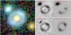 |
Fig. 8 Blue ring from the CFHTLS with a neighboring galaxy of a similar color in the observed projected plane (left panel). Without mask, sl_fit identifies this piece of environment as a bright lensed feature and searches for an incorrect lensing configuration (top right panel). Here, our standard masking eliminates most flux from the blue galaxy and thus helps the modeling to focus on the actual lensed flux (bottom right panel). As in Fig. 5, we show in each case the original image where the deflector has been subtracted in the g band, and the gravitational arcs or ring reconstructed by the model with the critical lines (in red). |
To mitigate these problems, we masked out of the input image all pixels at distances smaller than  and beyond
  . We hence assume that the multiple images (arcs, rings) nestle inside this thick annulus. This masking was performed after the deflector subtraction by galfit and only concerns the subsequent sl_fit fitting. As for simulated data, the fitting window is on a side. We chose to replace pixel values with pure noise realizations of zero mean and variance given by the input weight map. Hence lensed features appearing beyond were chopped off and not properly modeled. As an alternative, we explored the possibility to simply neglect these masked pixels in the χ2 calculation, which would not prevent the model from producing multiple images beneath the masked area. Moreover, by carrying out the fitting on a smaller number of pixels, the convergence of the chain is expected to occur faster. There still is a risk here of producing models far from the physical reality of some systems by conceiving arcs beyond that do not actually exist. Our experience suggested that the former approach was preferable if the goal is to avoid producing too many false large REin systems. Figure 8 shows the example of an observed ring from the CFHTLS for which the application of this simple masking is successful in recovering a lens configuration much closer to the truth.
5.2.2. Comparison with published models of SL2S lenses
Sonnenfeld et al. (2013a) produced detailed lens models of several confirmed SL2S lenses that had been observed with Keck or VLT spectrographs to measure redshifts and stellar velocity dispersions (see also Sonnenfeld et al. 2013b, 2014). Some systems were analyzed with HST imaging, others were relying on the same CFHT data as we used here. The main difference resides in the level of refinement devoted to foregound light subtraction, to the accounting of neighboring objects, and to a much richer model for the background source which is pixelized, all aspects that we cannot currently afford within a fast modeling strategy. We can therefore assume that Sonnenfeld et al. models are somehow “the truth” for our present goal. The subscript “Son++” refers to the parameter values from these models.
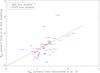 |
Fig. 9 Comparison between the Einstein radius REin measured by Sonnenfeld et al. (2013a) and our fast sl_fit inferences for 44 confirmed SL2S lenses. Sonnenfeld et al. models relying on HST (red) and CFHT (blue) images are distinguished. |
Figure 9 compares both estimates of REin for a sample of 44 systems out of the 517 SL2S candidates that we modeled. Here, we excluded a few cases that appeared to be especially complex, the observations suggesting peculiarities like a double deflector, a composite source hosting an AGN, a very bright piece of environment, etc. Moreover, the mask we decided to automatically apply to every candidate (see Sect. 5.2.1) affects lens systems with  by hiding substantial flux belonging to one or more lensed arcs, so we focused on systems such that
  for this comparison.
The scatter in the REin ↔ REinSon + + relation for HST models, given by 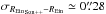 , is close to the
  value found for the simulations: this somehow proves the robustness of our REin estimate despite the new obstacles brought by real data. For CFHT data, the scatter is slightly larger
  . This value is mostly driven by three outliers for which the complete lack of visible counter image led the optimization to an unlikely lensing configuration: without these three, we derive the same satisfactory
  value as for HST models.
5.3. Calibrating sl_fit as an automated lens finder with real CFHTLS data: selection strategy
In Sect. 4, we have used a sample of 4260 simulated lens candidates of different classes, including unlensed galaxies, so as to maximize the purity rate of our selection while maintaining a reasonable completeness rate. For a galfit subtraction, the only previously addressed case that can be reproduced on real data, we finally achieved a purity rate of 69% and a rate of completeness of 31%. Using the preselected sample of 517 SL2S lens candidates, we now wish to recalibrate completeness and purity depending on the fraction of “real good lenses” that can be actually recovered by performing the same selection in the sl_fit output parameter space. Follow-up observations and minute modeling allowed a better assessment of the quality of a subset of SL2S candidates that were hence classified with a confirmed parameter taking values: “poor lenses” 0, “average lenses” 1, “good lenses” 2, and “excellent lenses” 3 (G14). For simplicity we merged “good” and “excellent” systems into a single class of “good” lenses. The RingFinder follow-up allowed constructing a transfer matrix (G14, Table 4) between the pre-follow-up quality flag q_flag and the confirmed parameter. Assuming that SL2S lenses that still lack confirmation (about 400) will obey the same q_flag→confirmed transfer matrix, we can assign a pseudo-confirmed value to all systems that do not have an actual confirmed value.
When applying the cuts defined in (8)6 and derived from the simulations to the real data, we get 50% of purity and only 7% of completeness, with respect to the parent RingFinder share between “good”, “average” and “poor” lenses. We thus note a slightly higher purity than for the straight 44% purity of the RingFinder sample. On the other hand, the relative completenes is very low. Concerning this result, one has to bear in mind that the selection applied here favors purity over completeness. Moreover, sl_fit modeling has a strong prejudice on the possible lens configurations: it is more demanding than RingFinder and will be less inclusive on real, potentially complex lenses. We recall that sl_fit modeling is really meant to improve the purity of strong lensing samples in the context of the very large surveys to come.
For now, this modest rate of completeness suggests that the previous selection should be broadened by updating our cuts on the sl_fit output parameter space of the real sample. This new selection is substantially simplified to avoid overlaps as much as possible. The distribution of sl_fit output parameters for CFHTLS lens candidates is shown in Fig. 10, where lines trace the following cuts in the {μ, mimg} subspace:  (9)
(9)
The previous 7% completeness value is noticeably enhanced since we now achieve a rate of 39% while leaving the purity rate unchanged around 52%, as reported in Table 4. Again, we stress that these values are relative to the parent sample preselected with RingFinder. A more accurate relative distribution between “good”, “average” and “poor” lenses should be found in the simulated sample. Indeed, calculations of purity and completeness with the new cuts favoring completeness of Eq. (9)give a different picture than for the previous cuts favoring purity of Eq. (8)and motivated by simulations. We now achieve 71% completeness for mock candidates, but the purity drops to 20%, as also reported in Table 4. Consequently, we see that a good compromise between completeness and purity remains difficult to achieve when dealing with a realistic deflector subtraction, as already mentioned in Sect. 3.2.
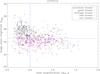 |
Fig. 10 Results of the sl_fit modeling of our real lens candidates in the {μ, mimg} subspace with a galfit subtraction of the deflector. Five classes of lenses are considered: “excellent lenses” (red), “good lenses” (pink), “average lenses” (green), “poor lenses” (blue), and “non-lenses” (black). This latter population is not part of the final RingFinder sample and is not considered for calculations. It has only been added to guide the eye to see where “non-lenses” should reside. Lines represent the simplified cuts that we applied to empirically isolate lenses. They are defined in Eq. (9). |
Updated selection results on real and simulated lens candidates.
6. Summary and conclusion
We have attempted to test whether a fast modeling of the light distribution around bright galaxies could provide a valuable diagnostic to decide whether a background source is strongly gravitationally lensed or not. We have shown that such a modeling and, consequently, such a diagnostic, are not trivial for ground-based observations, either for simulations of mock strong lensing events or from the CFHTLS survey itself. At present, the main limitation resides in subtracting the foreground light distribution. However, we have identified the most salient problems, and future progress could definitely foster the practical implementation of such a technique to the next generation of surveys.
With simulations of CFHTLS images in the g band from which the assumed deflector light was perfectly subtracted before the sl_fit analysis was performed, we have shown the following:
-
A fast modeling of ~10 s per system can satisfactorily recover the important input parameters, in particular the Einstein radius REin. This modeling is twice as fast as for the corresponding HST simulations.
-
Such a modeling allows precisely isolating lens systems in the {REin, β, μ, mimg, χ2/ν} output parameter space of sl_fit. From trying to favor purity over completeness at this stage, we estimate that 94% of purity and 82% of completeness could be achieved for lensing systems with an Einstein radius large enough, a sufficient magnification, bright lensed images, and a satisfactory fit. These correspond to Eq. (7).
For the more realistic situation in which the foreground light emission is removed by galfit, the picture is substantially degraded. We focused on ground-based simulations and found the following:
-
Despite an iterative red-to-blue fitting approach aimed at mitigating the effect of the lensed arcs on the fitting of the foreground galaxy, galfit often absorbs in its deflector model a large portion of the lensed light, thus hampering an accurate sl_fit fitting of the latter. The median execution time does not change compared to the ideal case.
-
The different classes of lens candidates are much more mixed up in the parameter space, which makes the good lenses much more difficult to isolate from the rest. Therefore, we could only come up with a more empirical selection as defined by Eq. (8). It provides samples that are 69% pure and 31% complete. We thus note a substantial loss in terms of selectivity due to our deflector subtraction method implying galfit.
We then applied our modeling and decision strategies to a subset of 517 SL2S lens candidates extracted from the CFHTLS survey.
-
When comparing our fast models to fine models from either HST or CFHT images that have been previously reported by Sonnenfeld et al. (2013a) for a subset of ~45 confirmed lenses, we find a good consistency between the relative estimations of the Einstein radius. This is an encouraging result since the robustness of the REin estimate is preserved despite the subtraction problems mentioned above and the increased complexity of real lenses that is lacking in our simulations (restricted to simple exponential sources, simple de Vaucouleurs deflectors, and perfect SIE lens potentials without neighboring objects along the line of sight).
-
When filtering this preselected sample through the set of cuts derived from the simulations, we achieve 50% of purity – which is a small gain compared to the 44% purity for the full original SL2S sample – and a low rate of completeness of 7%. We thus attempted to re-adjust the selection on the real data themselves: the simplified set of cuts given by Eq. (9)allows reaching 39% of completeness for a similar purity from the observed sample, but drives the purity down to 20% (for a completeness of 71%) when re-applied to the simulations.
-
Predictably, the completeness depends on the lens configurations: our modeling finder preferentially selects lenses with matter and light distributions close to our assumptions (see Sect. 2.1). This means that we might lose objects for which satellites or extra line-of-sight mass components add much complexity to the lens potential, as well as systems with an intrinsically complex deflector (like a double deflector) or source. Such cases indeed result in a complex image plane flux distribution, which leads to a chaotic likelihood surface. We do not expect the method to be much biased against multiple lenses since two lensed sources will give rise to two independent regions in the parameter space, providing a relative gain in χ2 (or log posterior) despite a poor absolute best-fit χ2. This is the reason why we did not apply stringent cuts on the fit quality. This essentially amounts to considering the benefit in χ2 of a model with a lensed source with respect to a model without it, regardless of how close this brings us to the theoretical floor predicted by our noise model. However, this needs to be better quantified with more realistic simulations of this kind of particularly interesting lenses (Gavazzi et al. 2008; Sonnenfeld et al. 2012; Collett & Auger 2014; Schneider 2014).
Consequently, the massive modeling part of our lens detection method, based on sl_fit, is efficient in recovering in a few seconds the most important parameters {REin, μ, mimg}. Because it encodes the lens equation, sl_fit modeling incorporates a valuable prior information in the lens-finding process (see also Marshall et al. 2009) and should therefore greatly improve purity (at the expense of complex lenses, however). In its present status, the method is mainly limited by the deflector subtraction, because galfit assigns flux from the lensed features to the deflector. This hampers an accurate sl_fit optimization which, in turn, prevents an effective selection of lenses in the sl_fit output parameter space. We foresee a number of options that should significantly improve the process in the near future:
-
We aim for sl_fit to be able to perform a simultaneous fit of the foreground light and of the lensed source in one or more photometric band(s). Coupling the problem of the deflector subtraction with the very lens modeling will allow fully understanding the complex cross-talk at work and, possibly, reducing some degeneracies. The multifilter approach has proven valuable in the RingFinder method (G14).
-
Instead of using a static 0–1 ring-shape mask around each potential deflector to mitigate the effect of neighboring objects on model fitting, we plan to use SExtractor (Bertin & Arnouts 1996) to detect and mask out one by one distant sources around the galaxies of interest. Although this appears to be simple, one should be cautious not to remove lensed features that are not well separated from the central deflector, as is usually the case. Multiple filters might also help here in distinguishing pieces of environment from lensed arcs of similar colors.
-
Like for the RingFinder algorithm (G14), a more realistic morphology of foreground deflectors should be included in our simulations since, in real data, we expect a fraction of false positives to arise from edge-on spirals or, more generally, from galaxies exhibiting satellites close to their center. This could be achieved by superimposing mock arcs on observed non-standard galaxies that are not actually lenses.
-
The execution time is quite short (about 10 s per system) from a modeling perspective, but remains too slow with a view toward lens finding in the context of future large-area surveys (all the more so if we aim for multiband simultaneous lens+source model-fitting). A preselection of potential lenses, in the vein of the ETG preselection of the SL2S sample considered here (see Sect. 5.1, and G14), will probably remain necessary. We also may have to abandon the benefits of MCMC posterior sampling and improve the straight minimization strategy we briefly mentioned in Sect. 2.4.2.
By simulating the same mock lenses under CFHT and HST conditions, we were able to estimate the benefit of space-based observations for the prospect of uncovering strong lenses. This is particularly relevant in the context of the future Euclid mission, and our HST simulations are very similar to what is expected with Euclid. This work suggests that the problem of foreground light subtraction is still present (although less prominent) with single-band well-resolved observations. It should therefore be cautiously addressed for Euclid. Promising methods are being developed (Joseph et al. 2014), but it remains to be shown whether they will not capture too much flux from the lensed features. Like for ground-based surveys, a multiband approach could break down the main barriers preventing massive lens modeling with Euclid and lead to a surge in the population of galaxy-scale strong lenses.
Acknowledgments
The authors would like to thank the anonymous referee for useful comments and their colleagues of the SL2S and SLACS collaborations for many useful discussions as well as stimulating exchanges within the Euclid Strong Lensing Science Working Group. R.G. also acknowledges E. Bertin for valuable discussions about massive model fitting. This work was supported by the Centre National d’Études Spatiales (CNES) and the Programme National Cosmologie et Galaxies (PNCG). This research is based on observations obtained with MegaPrime/MegaCam, a joint project of CFHT and CEA/DAPNIA, a joint project of CFHT, Taiwan, Korea, Canada and France, at the Canada-France-Hawaii Telescope (CFHT) which is operated by the National Research Council (NRC) of Canada, the Institut National des Sciences de l’Univers of the Centre National de la Recherche Scientifique (CNRS) of France, and the University of Hawaii. This work is based in part on data products produced at TERAPIX and the Canadian Astronomy Data Centre.
References
- Auger, M. W., Treu, T., Bolton, A. S., et al. 2010, ApJ, 724, 511 [NASA ADS] [CrossRef] [Google Scholar]
- Bertin, E., & Arnouts, S. 1996, A&AS, 117, 393 [NASA ADS] [CrossRef] [EDP Sciences] [Google Scholar]
- Bolton, A. S., Burles, S., Schlegel, D. J., Eisenstein, D. J., & Brinkmann, J. 2004, AJ, 127, 1860 [NASA ADS] [CrossRef] [Google Scholar]
- Bolton, A. S., Burles, S., Koopmans, L. V. E., Treu, T., & Moustakas, L. A. 2006, ApJ, 638, 703 [NASA ADS] [CrossRef] [Google Scholar]
- Bolton, A. S., Brownstein, J. R., Kochanek, C. S., et al. 2012, ApJ, 757, 82 [NASA ADS] [CrossRef] [Google Scholar]
- Brownstein, J. R., Bolton, A. S., Schlegel, D. J., et al. 2012, ApJ, 744, 41 [NASA ADS] [CrossRef] [Google Scholar]
- Cabanac, R. A., Alard, C., Dantel-Fort, M., et al. 2007, A&A, 461, 813 [NASA ADS] [CrossRef] [EDP Sciences] [Google Scholar]
- Capak, P., Aussel, H., Ajiki, M., et al. 2007, ApJS, 172, 99 [NASA ADS] [CrossRef] [Google Scholar]
- Collett, T. E., & Auger, M. W. 2014, MNRAS, 443, 969 [NASA ADS] [CrossRef] [Google Scholar]
- Dye, S., Negrello, M., Hopwood, R., et al. 2014, MNRAS, 440, 2013 [NASA ADS] [CrossRef] [Google Scholar]
- Gavazzi, R., Treu, T., Rhodes, J. D., et al. 2007, ApJ, 667, 176 [NASA ADS] [CrossRef] [Google Scholar]
- Gavazzi, R., Treu, T., Koopmans, L. V. E., et al. 2008, ApJ, 677, 1046 [NASA ADS] [CrossRef] [Google Scholar]
- Gavazzi, R., Cooray, A., Conley, A., et al. 2011, ApJ, 738, 125 [NASA ADS] [CrossRef] [Google Scholar]
- Gavazzi, R., Treu, T., Marshall, P. J., Brault, F., & Ruff, A. 2012, ApJ, 761, 170 [NASA ADS] [CrossRef] [Google Scholar]
- Gavazzi, R., Marshall, P. J., Treu, T., & Sonnenfeld, A. 2014, ApJ, 785, 144 [NASA ADS] [CrossRef] [Google Scholar]
- Goranova, Y., Hudelot, P., Magnard, F., et al. 2009, The CFHTLS T0006 Release, Tech. rep., Terapix – Institut d’Astrophysique de Paris, http://terapix.iap.fr/cplt/T0006/T0006-doc.pdf [Google Scholar]
- Ilbert, O., Capak, P., Salvato, M., et al. 2009, ApJ, 690, 1236 [NASA ADS] [CrossRef] [Google Scholar]
- Jiang, G., & Kochanek, C. S. 2007, ApJ, 671, 1568 [NASA ADS] [CrossRef] [Google Scholar]
- Joseph, R., Courbin, F., Metcalf, R. B., et al. 2014, A&A, 566, A63 [NASA ADS] [CrossRef] [EDP Sciences] [Google Scholar]
- Koopmans, L. V. E., Treu, T., Bolton, A. S., Burles, S., & Moustakas, L. A. 2006, ApJ, 649, 599 [NASA ADS] [CrossRef] [Google Scholar]
- Krist, J. E., Hook, R. N., & Stoehr, F. 2011, in Optical Modeling and Performance Predictions V, ed. M. A. Kahan, SPIE, 8127 [Google Scholar]
- Lagattuta, D. J., Fassnacht, C. D., Auger, M. W., et al. 2010, ApJ, 716, 1579 [NASA ADS] [CrossRef] [Google Scholar]
- Laureijs, R., Gondoin, P., Duvet, L., et al. 2012, in SPIE Conf. Ser., 8442 [Google Scholar]
- Marshall, P., Blandford, R., & Sako, M. 2005, New Astron. Rev., 49, 387 [Google Scholar]
- Marshall, P. J., Treu, T., Melbourne, J., et al. 2007, ApJ, 671, 1196 [NASA ADS] [CrossRef] [Google Scholar]
- Marshall, P. J., Hogg, D. W., Moustakas, L. A., et al. 2009, ApJ, 694, 924 [NASA ADS] [CrossRef] [Google Scholar]
- More, A., Cabanac, R., More, S., et al. 2012, ApJ, 749, 38 [Google Scholar]
- Negrello, M., Hopwood, R., De Zotti, G., et al. 2010, Science, 330, 800 [NASA ADS] [CrossRef] [Google Scholar]
- Newton, E. R., Marshall, P. J., & Treu, T. 2009, ApJ, 696, 1125 [NASA ADS] [CrossRef] [Google Scholar]
- Oguri, M., Rusu, C. E., & Falco, E. E. 2014, MNRAS, 439, 2494 [NASA ADS] [CrossRef] [Google Scholar]
- Peng, C. Y., Ho, L. C., Impey, C. D., & Rix, H.-W. 2002, AJ, 124, 266 [NASA ADS] [CrossRef] [Google Scholar]
- Peng, C. Y., Ho, L. C., Impey, C. D., & Rix, H.-W. 2010, AJ, 139, 2097 [NASA ADS] [CrossRef] [Google Scholar]
- Ruff, A. J., Gavazzi, R., Marshall, P. J., et al. 2011, ApJ, 727, 96 [NASA ADS] [CrossRef] [Google Scholar]
- Rusin, D., Kochanek, C. S., & Keeton, C. R. 2003, ApJ, 595, 29 [NASA ADS] [CrossRef] [Google Scholar]
- Schneider, P. 2014, A&A, 568, L2 [NASA ADS] [CrossRef] [EDP Sciences] [Google Scholar]
- Sonnenfeld, A., Treu, T., Gavazzi, R., et al. 2012, ApJ, 752, 163 [NASA ADS] [CrossRef] [Google Scholar]
- Sonnenfeld, A., Gavazzi, R., Suyu, S. H., Treu, T., & Marshall, P. J. 2013a, ApJ, 777, 97 [NASA ADS] [CrossRef] [Google Scholar]
- Sonnenfeld, A., Treu, T., Gavazzi, R., et al. 2013b, ApJ, 777, 98 [NASA ADS] [CrossRef] [Google Scholar]
- Sonnenfeld, A., Treu, T., Marshall, P. J., et al. 2014, ApJ, 800, 94 [Google Scholar]
- Treu, T. 2010, ARA&A, 48, 87 [NASA ADS] [CrossRef] [Google Scholar]
- Treu, T., & Koopmans, L. V. E. 2002a, ApJ, 575, 87 [NASA ADS] [CrossRef] [Google Scholar]
- Treu, T., & Koopmans, L. V. E. 2002b, MNRAS, 337, L6 [NASA ADS] [CrossRef] [Google Scholar]
- Treu, T., & Koopmans, L. V. E. 2004, ApJ, 611, 739 [NASA ADS] [CrossRef] [Google Scholar]
- Vieira, J. D., Marrone, D. P., Chapman, S. C., et al. 2013, Nature, 495, 344 [NASA ADS] [CrossRef] [Google Scholar]
- Wardlow, J. L., Cooray, A., De Bernardis, F., et al. 2013, ApJ, 762, 59 [NASA ADS] [CrossRef] [Google Scholar]
All Tables
All Figures
|
Fig. 1 Mosaic of six simulated gravitational lenses under CFHT (gri-color, left) and HST/WFPC2 (gray-scale, right) conditions. Each panel is |
| In the text | |
|
Fig. 2 Recovery of Einstein radius (top), total image-plane-lensed flux (middle), and magnification (bottom) for simulated lenses fitted with sl_fit in fast-modeling mode. We distinguish the case of ground-based CFHTLS-Wide-like g-band observations (left) and the case of HST WFPC2/F606W observations (right). In both cases, the deflector light has been “perfectly” subtracted before modeling the residual lensed features. In each panel, the red error bars show the binned median values for guidance. |
| In the text | |
|
Fig. 3 Recovery of the deflector g-band flux when fitted with galfit on CFHT (left) and HST (right) simulations, colored according to the initial magnitude of the lensed light. The lensed background component is oversubtracted in most cases. |
| In the text | |
|
Fig. 4 Recovery of Einstein radius (top), total image-plane-lensed flux (middle), and magnification (bottom) for simulated lenses fitted with sl_fit in fast-modeling mode. We distinguish the case of ground-based CFHTLS-wide-like g-band observations (left) and the case of HST WFPC2/F606W observations (right). In both cases, the deflector light has been subtracted with galfit before modeling the residuals. In this case, oversubtracted background emission or undersubtraction or inaccurate modeling of the deflector produces larger errors and biases on fitted important parameters of the lens models. In each panel, the red error bars show the binned median values for guidance. |
| In the text | |
|
Fig. 5 Comparative modeling of a simulated ring in the four cases considered in Sect. 3. Top panels: mock observations of the lens system under CFHT (gri-color, left) and HST/WFPC2 (gray-scale, right) conditions. Other panels: images where the deflector has been subtracted ideally (middle panels) or using galfit (bottom panels), along with the lensed features reconstructed by the model and the critical lines (in red). The CFHT simulations are modeled in the g band. Each panel is |
| In the text | |
|
Fig. 6 Results of the sl_fit modeling in the {REin, β} (top), {REin, μ} (middle), and {REin, mimg} (bottom) subspaces for an ideal subtraction of the deflector. Three classes of systems are considered: “good lenses” defined by μ0> 4 (pink), “average lenses” such that 2 <μ0< 4 (green), and galaxies that are not lenses (black). Lines represent the empirical cuts applied to isolate lenses. They are defined in Eq. (7). |
| In the text | |
|
Fig. 7 Same as Fig. 6, but for a galfit subtraction of the deflector. Lines represent the cuts defined in Eq. (8). |
| In the text | |
|
Fig. 8 Blue ring from the CFHTLS with a neighboring galaxy of a similar color in the observed projected plane (left panel). Without mask, sl_fit identifies this piece of environment as a bright lensed feature and searches for an incorrect lensing configuration (top right panel). Here, our standard masking eliminates most flux from the blue galaxy and thus helps the modeling to focus on the actual lensed flux (bottom right panel). As in Fig. 5, we show in each case the original image where the deflector has been subtracted in the g band, and the gravitational arcs or ring reconstructed by the model with the critical lines (in red). |
| In the text | |
|
Fig. 9 Comparison between the Einstein radius REin measured by Sonnenfeld et al. (2013a) and our fast sl_fit inferences for 44 confirmed SL2S lenses. Sonnenfeld et al. models relying on HST (red) and CFHT (blue) images are distinguished. |
| In the text | |
|
Fig. 10 Results of the sl_fit modeling of our real lens candidates in the {μ, mimg} subspace with a galfit subtraction of the deflector. Five classes of lenses are considered: “excellent lenses” (red), “good lenses” (pink), “average lenses” (green), “poor lenses” (blue), and “non-lenses” (black). This latter population is not part of the final RingFinder sample and is not considered for calculations. It has only been added to guide the eye to see where “non-lenses” should reside. Lines represent the simplified cuts that we applied to empirically isolate lenses. They are defined in Eq. (9). |
| In the text | |
Current usage metrics show cumulative count of Article Views (full-text article views including HTML views, PDF and ePub downloads, according to the available data) and Abstracts Views on Vision4Press platform.
Data correspond to usage on the plateform after 2015. The current usage metrics is available 48-96 hours after online publication and is updated daily on week days.
Initial download of the metrics may take a while.