| Issue |
A&A
Volume 561, January 2014
|
|
|---|---|---|
| Article Number | A84 | |
| Number of page(s) | 17 | |
| Section | Astrophysical processes | |
| DOI | https://doi.org/10.1051/0004-6361/201322829 | |
| Published online | 06 January 2014 | |
Dynamical friction in a gas: The supersonic case⋆
Astronomy DepartmentUniversity of California,
Berkeley,
CA
94720,
USA
e-mail:
sstahler@astro.berkeley.edu
Received:
10
October
2013
Accepted:
8
November
2013
Any gravitating mass traversing a relatively sparse gas experiences a retarding force created by its disturbance of the surrounding medium. In a previous contribution, we determined this dynamical friction force when the object’s velocity was subsonic. We now extend our analysis to the supersonic regime. As before, we consider small perturbations created in the gas far from the gravitating object, and thereby obtain the net influx of linear momentum over a large, bounding surface. Various terms in the perturbation series formally diverge, necessitating an approximate treatment of the flow streamlines. Nevertheless, we are able to derive exactly the force itself. As in the subsonic case, we find that F = Ṁ V , where Ṁ is the rate of mass accretion onto the object and V its instantaneous velocity with respect to distant background gas. Our force law holds even when the object is porous (e.g., a galaxy) or is actually expelling mass in a wind. Quantitatively, the force in the supersonic regime is less than that derived analytically by previous researchers, and is also less than was found in numerical simulations through the mid-1990s. We urge simulators to revisit the problem using modern numerical techniques. Assuming our result to be correct, it is applicable to many fields of astrophysics, ranging from exoplanet studies to galactic dynamics.
Key words: hydrodynamics / waves / ISM: kinematics and dynamics / planet-disk interactions / galaxies: kinematics and dynamics
Appendix A is available in electronic form at http://www.aanda.org
© ESO, 2014
1. Introduction
Whenever a massive object passes through a rarefied medium, it draws surrounding matter toward it. As a result, this material creates an overdense wake behind the object that exerts its own gravitational pull, retarding the original motion. Such dynamical friction arises whether the medium consists of non-interacting point particles, e.g., a stellar cluster, or a continuum fluid, e.g., an interstellar cloud. Chandrasekhar (1943) provided the essential theory when the background is collisionless, and his solution has been extensively used in studies of both star clusters and galaxies. Interaction of a gravitating object with gas also occurs in a wide variety of situations. A partial list of topics and references includes: the interaction of planets and gaseous disks (Teyssandier et al. 2013); the orbital decay of common-envelope binaries (Ricker & Taam 2008); the settling of massive stars in dense molecular clouds (Chavarría et al. 2010); the coalescence of massive black holes in both isolated galactic nuclei (Narayan 2000) and colliding galaxies (Armitage & Natarajan 2005); and the heating of intracluster gas by infalling galaxies (El-Zant et al. 2004).
Despite the widespread occurrence of gaseous dynamical friction, there is still no generally accepted derivation of the force, even after 70 years of effort. The flow in the vicinity of the gravitating mass is complex both temporally and spatially, as many simulations have shown (see, e.g. Matsuda et al. 1987). Theorists seeking a fully analytic expression for the time-averaged force have employed various strategems to circumvent a detailed description of this region. In the course of their classic studies of stellar accretion, Bondi & Hoyle (1944) took the star to be traversing a zero-temperature gas. In their model, fluid elements follow hyperbolic orbits in the star’s reference frame and land in an infinitely thin, dense spindle behind the object. Bondi & Hoyle analyzed the transfer of linear momentum from the spindle to the star, and hence obtained the force. Dodd & McCrae (1952) similarly investigated this hypersonic limit, as did, much more recently, Cantó et al. (2011). Dokuchaev (1964) first treated a finite-temperature gas. He determined the force by integrating the total power emitted by the object in acoustic waves (see also Rephaeli & Salpeter 1980). Ruderman & Spiegel (1971) used an impulse approximation in the reference frame of the background gas. Finally, Ostriker (1999) calculated the force by integrating directly over the wake, whose density she obtained through a linear perturbation analysis.
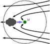 |
Fig. 1 Sketch of mass and momentum flow. Surrounding the central gravitating body of mass M is a large, imaginary sphere. The thin curves represent streamlines of background gas. After entering the sphere, most gas simply exits again, while a small portion joins directly onto the mass. In addition, some gas temporarily forms an overdense wake, also sketched here. The wake tugs gravitationally on the mass, thereby imparting momentum to it (broad arrow). All gas entering the wake also leaves it, either joining the mass or exiting the sphere. |
These researchers focused principally on the supersonic case, which is often the most interesting one astrophysically. That is, they took V > cs , where V is the speed of the gravitating mass relative to the distant background, and cs the sound speed in that gas. (In the hypersonic calculations of Bondi, Hoyle, and their successors, cs was implicitly set to zero.) While their answers differed in detail, all agreed that the friction force in this regime varies as V-2, with a coefficient that includes a Coulomb logarithm. This latter term also appears in the force derived by Chandrasekhar (1943), and arises from an integration in radius away from the mass. In all derivations, at least one of the integration limits is rather ill-defined.
The previous studies made two important, simplifying assumptions. First, they neglected any accretion of background gas by the moving object. Quantitatively, the assumption was that R ≫ racc , where R is the object’s physical radius and the accretion radius racc ≡ 2 G M/V2is the distance from the mass M within which its gravity qualitatively alters the background flow. They further ignored R compared to the scale for spatial variations in the surrounding flow. If L denotes the latter scale, then these assumptions may be summarized as L ≫ R ≫ racc . Unfortunately, the inequality R ≫ raccis often not satisfied. For example, a low-mass star moving through a cluster-producing molecular cloud has R ~ 1011 cmand racc ~ 1016 cm . An analysis that covers this regime should treat the object as being point-like in all respects, allowing the possibility of mass accretion through infall.
This infall cannot occur via direct impact, since the geometrical cross section of the body is negligible by assumption. Instead, some fluid elements that initially miss the object are pulled back into it. Mass accretion is, in fact, closely related to dynamical friction. In the reference frame attached to the mass, the background gas flows by with a speed that approaches V far away. The steady-state accretion rate onto the object is simply the net influx of mass through any closed surface surrounding it. Similarly, the friction force is the net influx of linear momentum. Much closer to the mass, this momentum influx manifests itself as two distinct force components. One is the gravitational pull from the wake, as described earlier. A second component is the direct advection of linear momentum from any background gas that falls into the object. Any determination of the force by an asymptotic surface integration cannot tease apart these two contributions.
To clarify these ideas, Fig. 1 shows graphically the mass and momentum flow within the extended gas cloud surrounding the central, gravitating object. Gas enters the region via the dotted sphere shown in the sketch. This gas then follows one of three paths. Most of it leaves the sphere downstream of the gravitating mass, as shown by the two outermost streamlines (thin solid curves). Only a small fraction of the gas makes its way to the deep interior. Some of it accretes onto the mass, first missing it and then looping back. Other gas that misses more widely is temporarily slowed by the gravitational pull of the mass and forms an overdense wake, also sketched in the figure. In steady state, the wake cannot gain net mass, so all of the gas entering it also leaves, either by joining onto the mass or exiting the sphere directly. Meanwhile, the wake itself tugs on the mass gravitationally. The broad arrow in the figure depicts this second form of momentum input to the mass. It is possible to determine the force analytically by integrating the net momentum flux over the bounding sphere. Numerical simulations can obtain this same force by calculating the advective and gravitational components acting directly on the mass.
In a previous paper (Lee & Stahler 2011, hereafter Paper I), we did the analytic surface integration. We focused on the subsonic case, V < cs , which traditionally has been less explored1. Working in the reference frame whose origin is attached to the mass, we developed a perturbative method to analyze the small deviations of the background gas from a uniform, constant-density, flow. By integrating the perturbed variables over a large sphere to obtain the net momentum influx, we arrived at a surprisingly simple result for the force: F = Ṁ V . Here, Ṁ is the mass accretion rate onto the moving object. To evaluate this quantity from first principles, one would have to follow the trajectories of fluid elements as they accrete onto the central mass, and ensure that, following turnaround, they smoothly cross the sonic transition. This transition occurs well inside the region of validity for our calculation. Lacking a fundamental theory for Ṁ, we adopted a variant of the interpolation formula of Bondi (1952) and thus found the force explicitly as a function of velocity. In this subsonic regime, our expression agrees reasonably well with past simulations (e.g., Ruffert 1996).
Here we apply the same technique to study the supersonic case. We quickly encounter the technical difficulty that some perturbation variables diverge, when expressed as functions of the angle from the background velocity vector. The true flow around the gravitating mass is, of course, well-defined everywhere, and the divergences simply indicate that the adopted series expansions fail at certain locations. Despite this mathematical inconvenience, we are able once again to derive the dynamical friction force through spatial integration of the linear momentum influx. The force has exactly the same form as previously: F = Ṁ V . In the high-speed limit, we recover the V-2 behavior found by others, but not the Coulomb logarithm.
In Sect. 2 below, we describe our solution strategy, and then formulate the problem using a convenient, non-dimensional scheme. Whenever material repeats that of Paper I, we abbreviate its presentation as much as possible. Section 3 analyzes the perturbed flow to first order only. In this approximation, we find there is no mass accretion or friction force, just as in the subsonic case. We extend the analysis to second order in Sect. 4, thus accounting for mass accretion. Here we also describe our method for calculating the flow numerically, and show sample results. Section 5 presents the analytic derivation of the force itself, and compares our expression to past simulations. Those found a greater force than we derive in the supersonic regime; we indicate possible causes for this discrepancy. Assuming our result to be correct, we present several representative applications. Finally, Sect. 6 compares our derivation to previous ones, and indicates directions for future work.
2. Method of solution
2.1. Physical assumptions
In the reference frame whose origin coincides with the mass, the background gas has speed V far from the object and a spatially uniform density, which we denote as ρ0. We take the gas to be isothermal, with associated sound speed cs. As depicted in Fig. 2, we will be working in a spherical coordinate system (r,θ), and will assume that the gas flow is axisymmetric about the polar (z-) axis, which is parallel to the asymptotic fluid velocity.
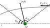 |
Fig. 2 Mathematical treatment of the flow. We erect a spherical coordinate system centered
on the gravitating body. The gas is isothermal, and its velocity far upstream is
β cs (β > 1).
Indicated are the Mach angle θM and its
supplement, |

We neglect the self-gravity of the gas, and will be analyzing perturbations to the flow
relatively far from the central mass. Specifically, our expansions are valid for
r ≫ rs , where
 is the sonic
radius. We assume that in the far-field region of interest, the flow is steady-state. Of
course, a steady flow cannot be established over arbitrarily large distances, and one must
judge, in each astrophysical situation, whether the assumption is justified. In numerical
simulations, which we later discuss by way of comparison, the flow occurs within some
fixed computational volume, at the center of which lies the mass. For the non-relativistic
case of relevance, the force of gravity propagates instantaneously, but alterations in the
flow density and velocity take time. In practice, a steady flow is indeed approached in
many such experiments (e.g., Pogorelov et al.
2000). The observed decay of transients is instructive, but again is only broadly
suggestive of what may occur in Nature.
is the sonic
radius. We assume that in the far-field region of interest, the flow is steady-state. Of
course, a steady flow cannot be established over arbitrarily large distances, and one must
judge, in each astrophysical situation, whether the assumption is justified. In numerical
simulations, which we later discuss by way of comparison, the flow occurs within some
fixed computational volume, at the center of which lies the mass. For the non-relativistic
case of relevance, the force of gravity propagates instantaneously, but alterations in the
flow density and velocity take time. In practice, a steady flow is indeed approached in
many such experiments (e.g., Pogorelov et al.
2000). The observed decay of transients is instructive, but again is only broadly
suggestive of what may occur in Nature.
Figure 2 singles out two special angles, both of
which only occur in supersonic flow. The first is the familiar Mach angle, defined through
the relation 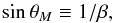 (1)where
β ≡ V/cs
. The second is the supplement of the first:
(1)where
β ≡ V/cs
. The second is the supplement of the first:  . The figure of
revolution swept out by the radius lying along
θ = θMis the Mach cone,
while we dub the analogous figure swept out by
. The figure of
revolution swept out by the radius lying along
θ = θMis the Mach cone,
while we dub the analogous figure swept out by  the
“anti-Mach cone”. As Fig. 3 illustrates, we denote as
the “upstream” region that portion of the flow bounded by the anti-Mach cone, while the
“downstream” region lies within the Mach cone. Finally, the “intermediate” region has
the
“anti-Mach cone”. As Fig. 3 illustrates, we denote as
the “upstream” region that portion of the flow bounded by the anti-Mach cone, while the
“downstream” region lies within the Mach cone. Finally, the “intermediate” region has
 .
.
 |
Fig. 3 Regions of the flow. The upstream and downstream regions lie within the anti-Mach and Mach cones, respectively. Between the two cones is the intermediate region. In the far-field flow, there are no physical barriers between the intermediate region and its neighbors, although mathematical divergences appear at the two cones. |
A significant feature of the flow surrounding a gravitating mass is the presence of an
accretion bowshock. Any fluid element that joins onto the mass penetrates to
r ≲ racc , and encounters a shock at
θ ~ θM . At much larger
r, such bowshocks weaken and degenerate to acoustic pulses, before
fading away entirely (Zel’dovich & Raizer
1968, Chap. 1). No such shock arises near  , even at
relatively small distances. In summary, for
r ≫ rs ≳ racc ,
we do not expect any discontinuities at θM or
in
steady-state flow, either in the fluid variables themselves or their derivatives. We need
to keep this key point in mind as we encounter apparent discontinuities at both angles.
, even at
relatively small distances. In summary, for
r ≫ rs ≳ racc ,
we do not expect any discontinuities at θM or
in
steady-state flow, either in the fluid variables themselves or their derivatives. We need
to keep this key point in mind as we encounter apparent discontinuities at both angles.
2.2. Mathematical formulation
As in Paper I, we describe the flow through two dependent variables, the mass density
ρ(r,θ) and the stream function
ψ(r,θ). Individual velocity components may be
recovered from these through the relations 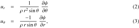 which
automatically ensure mass continuity. In the extreme far-field limit, the stream function
approaches that for the background, uniform flow:
which
automatically ensure mass continuity. In the extreme far-field limit, the stream function
approaches that for the background, uniform flow: 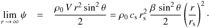 Our
second form of the stream function’s limit suggests how to expand
ψ(r,θ) in a perturbation series valid for finite, but
large, r:
Our
second form of the stream function’s limit suggests how to expand
ψ(r,θ) in a perturbation series valid for finite, but
large, r: ![\begin{eqnarray} \psi &=& \rho_0\,c_{\rm s}\,r_{\rm s}^2\,\left[ f_2\left(r\over r_{\rm s}\right)^2 + f_1\left(r\over r_{\rm s}\right) \,\right. +\,f_0+ \left. f_{-1}\left(r\over r_{\rm s}\right)^{-1} + ...\,\right] . \end{eqnarray}](/articles/aa/full_html/2014/01/aa22829-13/aa22829-13-eq41.png) (4)Here,
f2 ≡ β sin2θ/2
, while f1, f0,
f-1, etc., are as yet unknown, non-dimensional functions of
β and θ. We write a similar perturbation expansion for
the density:
(4)Here,
f2 ≡ β sin2θ/2
, while f1, f0,
f-1, etc., are as yet unknown, non-dimensional functions of
β and θ. We write a similar perturbation expansion for
the density: ![\begin{eqnarray} \rho &=& \rho_0\,\left[ 1 + g_{-1}\left({r\over r_{\rm s}}\right)^{-1} + g_{-2}\left({r\over r_{\rm s}}\right)^{-2} \, \right. \left. + g_{-3}\left({r\over r_{\rm s}}\right)^{-3} + ...\,\right] . \end{eqnarray}](/articles/aa/full_html/2014/01/aa22829-13/aa22829-13-eq48.png) (5)The
quantities g-1, g-2, and
g-3 are again non-dimensional functions of
β and θ, all of them unknown at this stage2.
(5)The
quantities g-1, g-2, and
g-3 are again non-dimensional functions of
β and θ, all of them unknown at this stage2.
The dynamical equations will be simplified once we recast all variables into
non-dimensional form. We let the fiducial radius, density, and speed be
rs, ρ0, and
cs, respectively, while we normalize the stream function to
 . We will
not change notation, but alert the reader whenever we revert to dimensional varables. Our
fully non-dimensional perturbation series are
. We will
not change notation, but alert the reader whenever we revert to dimensional varables. Our
fully non-dimensional perturbation series are ![\begin{eqnarray} \label{eqn:exppsi} \psi &=& f_2\ r^2 + f_1\ r + f_0 + f_{-1}\ r^{-1} + ... \\[2mm] \label{eqn:exprho} \rho &=& 1 + g_{-1}\ r^{-1} + g_{-2}\ r^{-2} + g_{-3}\ r^{-3} + ... \end{eqnarray}](/articles/aa/full_html/2014/01/aa22829-13/aa22829-13-eq54.png) The
task will be to solve for the various functions
fi(θ) and
gi(θ) appearing in these
two series. (Henceforth, we will suppress the β-dependence for
simplicity.) As explained in Sect. 2.3 of Paper I, the appropriate boundary conditions are
The
task will be to solve for the various functions
fi(θ) and
gi(θ) appearing in these
two series. (Henceforth, we will suppress the β-dependence for
simplicity.) As explained in Sect. 2.3 of Paper I, the appropriate boundary conditions are
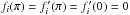 for
i = 1, 0, −1, −2 ,
etc., and fi(0) = 0for
i = 1, −1, −2 , etc. These
conditions ensure regularity of both ur and
uθ, as given by Eqs. (2) and (3),
respectively, on both the upstream and downstream axes. Since sinθ → 0 on
both axes, the r- and θ-derivatives of
ψ must also vanish. Using the expansion of ψ in Eq.
(6), we derive the aforementioned conditions. There is no associated restriction on
f0(0), which is tied to the mass accretion rate onto the
central object, as shown in Sect. 4 below.
for
i = 1, 0, −1, −2 ,
etc., and fi(0) = 0for
i = 1, −1, −2 , etc. These
conditions ensure regularity of both ur and
uθ, as given by Eqs. (2) and (3),
respectively, on both the upstream and downstream axes. Since sinθ → 0 on
both axes, the r- and θ-derivatives of
ψ must also vanish. Using the expansion of ψ in Eq.
(6), we derive the aforementioned conditions. There is no associated restriction on
f0(0), which is tied to the mass accretion rate onto the
central object, as shown in Sect. 4 below.
3. First-order flow
3.1. Upstream and downstream regions
The r- and θ-components of Euler’s equation, in non-dimensional form, are
![\begin{eqnarray} \label{eqn:rEuler} &&u_r\,{{\partial u_r}\over{\partial r}} + {u_\theta\over r}\, {{\partial u_r}\over{\partial\theta}} - {{u_\theta^2}\over r}= -{1\over\rho}\,{{\partial\rho}\over{\partial r}}\, -\,{1\over r^2} \\[2mm] \label{eqn:thetaEuler} &&u_r\,{{\partial u_\theta}\over{\partial r}} + {u_\theta\over r}\, {{\partial u_\theta}\over{\partial\theta}} + {{u_r\,u_\theta}\over r}= -{1\over{\rho\,r}}\,{{\partial\rho}\over{\partial\theta}}\cdot \end{eqnarray}](/articles/aa/full_html/2014/01/aa22829-13/aa22829-13-eq66.png) Our
procedure is first to express ur and
uθ in terms of ψ and
ρ, using Eqs. (2) and
(3). We then expand ψ
and ρ themselves in their respective perturbation series and equate the
coeffcients of various powers of r. To avoid cumbersome division by the
series for ρ, we first multiply Eqs. (8) and (9) through by
ρ3.
Our
procedure is first to express ur and
uθ in terms of ψ and
ρ, using Eqs. (2) and
(3). We then expand ψ
and ρ themselves in their respective perturbation series and equate the
coeffcients of various powers of r. To avoid cumbersome division by the
series for ρ, we first multiply Eqs. (8) and (9) through by
ρ3.
Equating the coefficients of the highest power of r, which is
r-1, we find that they are identically equal. Equating
coefficients of r-2 yields the first-order equations. From Eq.
(8), we find 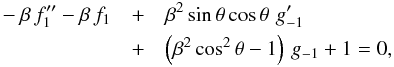 (10)while
Eq. (9) yields
(10)while
Eq. (9) yields  (11)These equations
are identical in form to Eqs. (18) and (19), respectively, of Paper I, hereafter
designated Eqs. (I.18) and (I.19). However, their solutions may differ. The factor
(1 − β2 sin2 θ)in Eq. (11), which was positive in the subsonic case
for any angle θ, can now be positive, negative, or zero.
(11)These equations
are identical in form to Eqs. (18) and (19), respectively, of Paper I, hereafter
designated Eqs. (I.18) and (I.19). However, their solutions may differ. The factor
(1 − β2 sin2 θ)in Eq. (11), which was positive in the subsonic case
for any angle θ, can now be positive, negative, or zero.
Consider first the upstream region. For  , the term
(1 − β2 sin2 θ)is indeed
positive, and we may recast Eq. (11) as
, the term
(1 − β2 sin2 θ)is indeed
positive, and we may recast Eq. (11) as
![\begin{eqnarray*} {{{\rm d}{\phantom \theta}}\over{{\rm d}\theta}} \left[\left(1 - \beta^2\,{\rm sin}^2\,\theta\right)^{1/2}\,g_{-1}\right]=0, \end{eqnarray*}](/articles/aa/full_html/2014/01/aa22829-13/aa22829-13-eq75.png) whose
solution is
whose
solution is 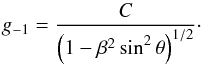 (12)Here, C
is independent of θ, but is possibly a function of β.
The analogous result appeared in our subsonic analysis as Eq. (I.20). In that case, we
ultimately found C to be unity.
(12)Here, C
is independent of θ, but is possibly a function of β.
The analogous result appeared in our subsonic analysis as Eq. (I.20). In that case, we
ultimately found C to be unity.
Returning to the supersonic flow, we see that, for any non-zero C, the
function g-1 diverges at
 . This fact
does not mean that the density itself diverges at that location; there is no reason for it
to do so. Rather, it is our series expansion of
ρ (r,θ) that fails in this region. The issue here is
mathematical, rather than physical. Although the function
g-1(θ) diverges, the associated term in the
perturbation expansion, Eq. (7), is
multiplied by r-1. At any finite angular separation from
, the
first-order correction to the background density can be made arbitrarily small by
considering a sufficiently large r-value. This observation suggests that
the divergences encountered here and elsewhere in our analysis will vanish if we change
independent variables from r and θ to another set that
mixes the two. In any case, we do not explore that possibility in the present paper.
. This fact
does not mean that the density itself diverges at that location; there is no reason for it
to do so. Rather, it is our series expansion of
ρ (r,θ) that fails in this region. The issue here is
mathematical, rather than physical. Although the function
g-1(θ) diverges, the associated term in the
perturbation expansion, Eq. (7), is
multiplied by r-1. At any finite angular separation from
, the
first-order correction to the background density can be made arbitrarily small by
considering a sufficiently large r-value. This observation suggests that
the divergences encountered here and elsewhere in our analysis will vanish if we change
independent variables from r and θ to another set that
mixes the two. In any case, we do not explore that possibility in the present paper.
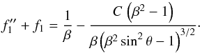
Substitution of Eq. (12) for
g-1 into (10)
yields the governing equation for f1:
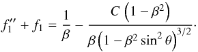 (13)This equation, being
identical to (I.21), has the same general solution:
(13)This equation, being
identical to (I.21), has the same general solution: 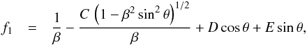 (14)where
D and E are additional constants. The vanishing of
f1 (π) tells us that
D = (1 − C)/β ,
while
(14)where
D and E are additional constants. The vanishing of
f1 (π) tells us that
D = (1 − C)/β ,
while  implies that
E = 0 . Both relations also held in the subsonic case.
implies that
E = 0 . Both relations also held in the subsonic case.
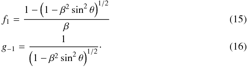
We next turn to the downstream region. Here again, the critical term (1 − β2 sin2 θ)is positive. The solutions for g-1 and f1 are thus identical to the upstream solutions in Eqs. (12) and (14), if we replace C, D, and E by new constants C′, D′, and E′. Application of the appropriate boundary conditions then tells us that E′ = 0and D′ = (C′ − 1)/β .
Referring again to Fig. 3, the supersonic flow we are now analyzing differs from the subsonic one by the presence of the intermediate region, lying between the Mach and anti-Mach cones. As β decreases to unity from above, this region narrows symmetrically about θ = π/2and ultimately vanishes, as does the physical distinction between the supersonic and subsonic flows. Continuity strongly suggests that, while (C,D)and (C′,D′)could, in principle, be β-dependent, they are actually not. Instead, they have the truly constant values (1,0)found in the subsonic case.
In summary, the first-order flow in both the upstream and downstream regions is described by
 After
substituting these coefficients into the series expansions for ψ and
ρ, one may calculate ur
and uθ to linear order from Eqs. (2) and (3), respectively. At any fixed, r-value, however, the series
representation for ρ fails sufficiently close to either Mach cone, and
the velocity components cannot be obtained in this manner.
After
substituting these coefficients into the series expansions for ψ and
ρ, one may calculate ur
and uθ to linear order from Eqs. (2) and (3), respectively. At any fixed, r-value, however, the series
representation for ρ fails sufficiently close to either Mach cone, and
the velocity components cannot be obtained in this manner.
Comparing our results thus far with the previous literature, Dokuchaev (1964); Ruderman & Spiegel (1971); and Ostriker (1999) all obtained Eq. (12) for the downstream, first-order density distribution, but with C = 2 . They also found that g-1 vanishes for θ > θM . In the subsonic analysis of Ostriker (1999), g-1 is everywhere finite. Thus, the density distributions in her supersonic and subsonic flows do not approach one another in the β = 1limit. Ruderman & Spiegel (1971) further argued that the apparent divergence in the downstream density perturbation at θ = θMsignifies the presence of a bowshock. While a bowshock certainly arises relatively close to the gravitating mass, it does not persist into the far field, the only regime where an analysis based on small perturbations of the background gas is justified.
3.2. Intermediate region
For  , the term
(1 − β2 sin2 θ)in Eq. (11) is negative. We therefore rewrite this
equation as
, the term
(1 − β2 sin2 θ)in Eq. (11) is negative. We therefore rewrite this
equation as  (17)This is equivalent
to
(17)This is equivalent
to ![\begin{eqnarray*} {{{\rm d}{\phantom \theta}}\over{{\rm d}\theta}} \left[\left(\beta^2\,{\rm sin}^2\,\theta - 1\right)^{1/2}\,g_{-1}\right] = 0 , \end{eqnarray*}](/articles/aa/full_html/2014/01/aa22829-13/aa22829-13-eq104.png) which
in turn implies that
which
in turn implies that 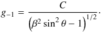 (18)Here we are reverting to
our original notation for the integration constants, as the previous ones have all been
evaluated.
(18)Here we are reverting to
our original notation for the integration constants, as the previous ones have all been
evaluated.
Substitution of the new expression for g-1 into Eq. (10) yields
 (19)We may solve this
equation using the method of variation of parameters. Adding the two homogeneous solutions
yields the general result
(19)We may solve this
equation using the method of variation of parameters. Adding the two homogeneous solutions
yields the general result 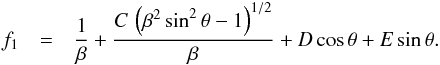 (20)As
in the upstream and downstream regions, the series representation of ψ is
well-behaved at either Mach cone, at least to linear order. Approaching either cone from
the outside, Eq. (15) tells us that
f1 → 1/β . Equation
(20) above implies that
f1 has the additional term
D cos θ + E sin θwhen
we approach the cones from the intermediate region.
(20)As
in the upstream and downstream regions, the series representation of ψ is
well-behaved at either Mach cone, at least to linear order. Approaching either cone from
the outside, Eq. (15) tells us that
f1 → 1/β . Equation
(20) above implies that
f1 has the additional term
D cos θ + E sin θwhen
we approach the cones from the intermediate region.
To proceed, we consider the physical interpretation of the stream function. Equation (2) tells us that ψ(r,θ) is the θ-integral of the mass flux ρ ur over a surface of radius r. More generally, the stream function is the net rate of mass transport into any surface of revolution extending from θ = 0to the angle of interest. A discontinuity in ψ at an angle θ thus represents a thin sheet of mass being injected or ejected along the corresponding cone. If we are to reject such a solution as unphysical, then we must demand continuity of ψ. That is, f1 must again approach 1/β at the two Mach cones, and D = E = 0in Eq. (20).
Our mathematical description of the first-order flow in the intermediate region is now
![\begin{eqnarray} \label{eqn:fFOiC2} &&f_1 = {{1 + C\,\left(\beta^2\,{\rm sin}^2\,\theta - 1\right)^{1/2}} \over\beta} \\[2mm] \label{eqn:gFOiC2} &&g_{-1} = {C\over{\left(\beta^2\,{\rm sin}^2\,\theta - 1\right)^{1/2}}} \cdot \end{eqnarray}](/articles/aa/full_html/2014/01/aa22829-13/aa22829-13-eq114.png) Since
the intermediate region does not reach either the upstream or downstream axis, we cannot
appeal to our usual boundary conditions in order to evaluate C. We defer
this issue until our analysis of the second-order flow in Sect. 4, when we will show that
the requirement of mass continuity again settles the matter. For any
C-value, the divergence of g-1 at the Mach
and anti-Mach cones indicates a breakdown of the series representation for the density.
Since
the intermediate region does not reach either the upstream or downstream axis, we cannot
appeal to our usual boundary conditions in order to evaluate C. We defer
this issue until our analysis of the second-order flow in Sect. 4, when we will show that
the requirement of mass continuity again settles the matter. For any
C-value, the divergence of g-1 at the Mach
and anti-Mach cones indicates a breakdown of the series representation for the density.
3.3. Vorticity
A key, simplifying property of the flow is that it is irrotational. To reprise the
argument from Paper I, we first write Euler’s equation in the steady state as
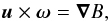 (23)where
ω ≡ ∇ × uis
the vorticity and the Bernoulli function on the right-hand side is
(23)where
ω ≡ ∇ × uis
the vorticity and the Bernoulli function on the right-hand side is  (24)Dotting both sides
of Eq. (23) with
u, we find that
(24)Dotting both sides
of Eq. (23) with
u, we find that  which
is the familiar statement that B is constant along streamlines. Moreover,
B approaches β2/2 at
large r, both upstream and downstream. (Recall that the non-dimensional
density ρ becomes unity in this limit.) In these regions, therefore,
B has the same value on every streamline, and
∇B = 0 . Since ω is
orthogonal to u in our poloidal flow, Eq. (23) imples that
ω = 0 , i.e., the flow is irrotational outside the Mach
cones.
which
is the familiar statement that B is constant along streamlines. Moreover,
B approaches β2/2 at
large r, both upstream and downstream. (Recall that the non-dimensional
density ρ becomes unity in this limit.) In these regions, therefore,
B has the same value on every streamline, and
∇B = 0 . Since ω is
orthogonal to u in our poloidal flow, Eq. (23) imples that
ω = 0 , i.e., the flow is irrotational outside the Mach
cones.
If our derived intermediate solution is correct, then irrotationality must hold there as
well, since there is no physical barrier between the intermediate flow and those upstream
and downstream, at least in the laminar, far field. The only non-zero component of the
vorticity is ωφ, so the condition of
irrotationality becomes  (25)To test the validity of
this relation in the intermediate region, we use Eqs. (2) and (3) for
ur and
uθ, respectively, and then substitute in
the series expansions for ψ and ρ, Eqs. (6) and (7).
(25)To test the validity of
this relation in the intermediate region, we use Eqs. (2) and (3) for
ur and
uθ, respectively, and then substitute in
the series expansions for ψ and ρ, Eqs. (6) and (7).
Equating the coefficient of the highest power of r, which is
r0, is equivalent to testing for irrotationality in the
uniform, background flow. Specifically, we require  (26)Using
f2 = β sin2 θ/2
, we verify that the above equation does hold. This result is to be expected, as a uniform
flow is manifestly irrotational.
(26)Using
f2 = β sin2 θ/2
, we verify that the above equation does hold. This result is to be expected, as a uniform
flow is manifestly irrotational.
We next equate the coefficients of r-1, effectively testing
irrotationality in the first-order flow. The required condition is now  (27)where
f1 and g-1 are given by Eqs.
(21) and (22), respectively. Using these functional forms, we find that this
last equation is satisfied for any value of C. Thus, the first-order flow
in the intermediate region is indeed irrotational.
(27)where
f1 and g-1 are given by Eqs.
(21) and (22), respectively. Using these functional forms, we find that this
last equation is satisfied for any value of C. Thus, the first-order flow
in the intermediate region is indeed irrotational.
4. Second-order flow
4.1. Dynamical equations
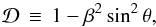
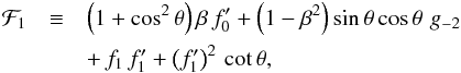
Having established the first-order flow, at least up to the constant C, we consider the next higher approximation. We return to the perturbative expansion of Euler’s equation, as described at the beginning of Sect. 3.1. By equating coefficients of r-3, we derive the second-order equations, which govern the variables f0 and g-2. Here the source terms involve f1 and g-1. Prior to substituting in the explicit solutions for f1 and g-1, the equations are identical to those in the subsonic problem; we display them again for convenient reference.
From the r-component of Euler’s equation, we derive Eq. (I.27), which is
 (28)The
three right-hand terms are
(28)The
three right-hand terms are ![\begin{eqnarray*} {\cal A}_1 &\equiv& {f_1^2\over{{\rm sin}^2\,\theta}} - {{f_1\,f_1^\prime\,{\rm cos}\,\theta}\over{{\rm sin}^3\,\theta}} + {{\left(f_1^\prime\right)^2}\over{{\rm sin}^2\,\theta}} + {{f_1\,f_1^{\prime\prime}}\over{{\rm sin}^2\,\theta}} \\[2mm] {\cal A}_2 &\equiv& \beta\,f_1\,\,g_{-1} - 2\,\beta\,f_1^\prime\,\,g_{-1}\,{\rm cot}\,\theta - \beta\,f_1\,\,g_{-1}^\prime\,{\rm cot}\,\theta - \beta\,f_1^\prime\,\,g_{-1}^\prime \\ &&+\, \beta\,f_1^{\prime\prime}\,\,g_{-1} \\ {\cal A}_3 &\equiv& 2\,g_{-1}^2 - 3\,g_{-1} . \end{eqnarray*}](/articles/aa/full_html/2014/01/aa22829-13/aa22829-13-eq133.png) The
θ-component of Euler’s equation yields Eq. (I.31):
The
θ-component of Euler’s equation yields Eq. (I.31):  (29)Here,
 (30)and
 In
the upstream and downstream regions, there are no unknown constants in the source terms,
i.e., both f1 and g-1 are
identical to their subsonic counterparts. Hence, the explicit form of the second-order
equations is also the same. Referring to Eqs. (I.35) and (I.36), we have
In
the upstream and downstream regions, there are no unknown constants in the source terms,
i.e., both f1 and g-1 are
identical to their subsonic counterparts. Hence, the explicit form of the second-order
equations is also the same. Referring to Eqs. (I.35) and (I.36), we have 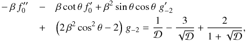 (31)and
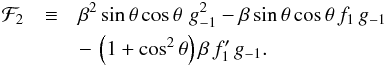
![\begin{eqnarray} \label{eqn:thetaSOu} -\beta\,f_0^\prime &+& {\cal D}\,g_{-2}^\prime - 2\,\beta^2\,{\rm sin}\,\theta\,\,{\rm cos}\,\theta\,\,g_{-2} \nonumber \\[2.5mm] &=& \beta^2\,{\rm sin}\,\theta\,\,{\rm cos}\,\theta \left[-{2\over{{\cal D}^2}} + {2\over{{\cal D}^{3/2}}}\,\right. -\left. {1\over{\cal D}} + {1\over{\left(1+\sqrt{\cal D}\right)^2}} \right]\cdot \end{eqnarray}](/articles/aa/full_html/2014/01/aa22829-13/aa22829-13-eq138.png) (32)In
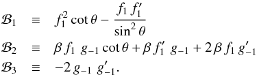
the intermediate region, however, f1 and
g-1 are given by the new expressions in Eqs. (21) and (22), respectively. After lengthy manipulation, we find the new source
terms, and hence the explicit dynamical equations in this region. These equations, which
still contain the unknown constant C, are
(32)In
the intermediate region, however, f1 and
g-1 are given by the new expressions in Eqs. (21) and (22), respectively. After lengthy manipulation, we find the new source
terms, and hence the explicit dynamical equations in this region. These equations, which
still contain the unknown constant C, are
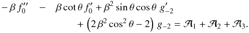
![\begin{eqnarray} \label{eqn:rSOi} &&-\,\, \beta\,f_0^{\prime\prime} - \beta\,{\rm cot}\,\theta\,f_0^\prime + \beta^2\,{\rm sin}\,\theta\,{\rm cos}\,\theta\,\,g_{-2}^\prime + \left(2\,\beta^2\,{\rm cos}^2\,\theta - 2\right)\,g_{-2}=\nonumber\\[2.5mm] &&{{2\,C\,{\cal E}^{1/2}}\over{\beta^2\,{\rm sin}^2\,\theta}} -{{3\,C}\over{{\cal E}^{1/2}}} + {C^2\over{\cal E}} + {{1 - C^2}\over{\beta^2\,{\rm sin}^2\,\theta}} , \end{eqnarray}](/articles/aa/full_html/2014/01/aa22829-13/aa22829-13-eq139.png) (33)and
(33)and
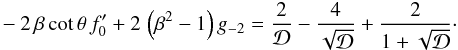
![\begin{eqnarray} \label{eqn:thetaSOi} &&-\,\,\beta\,f_0^\prime - {\cal E}\,g_{-2}^\prime - 2\,\beta^2\,{\rm sin}\,\theta\,\,{\rm cos}\,\theta\,\,g_{-2}= \,\nonumber\\[2.5mm] && {{2\,C^2\,\beta^2\,{\rm sin}\,\theta\,{\rm cos}\,\theta}\over{{\cal E}^2}} - {{2\,C\,\beta^2\,{\rm sin}\,\theta\,{\rm cos}\,\theta}\over{\cal E}^{3/2}} \nonumber\\[2.5mm] &&-\,\, {{C^2\,\beta^2\,{\rm sin}\,\theta\,{\rm cos}\,\theta}\over{\cal E}} +{{\left(1-C^2\right){\rm cot}\,\theta}\over{\beta^2\,{\rm sin}^2\,\theta}} \nonumber\\[2.5mm] &&+\,\, C^2\,{\rm cot}\,\theta +\,{{2\,C\,{\cal E}^{1/2}\,{\rm cot}\,\theta}\over{\beta^2\,{\rm sin}^2\,\theta}}\cdot \end{eqnarray}](/articles/aa/full_html/2014/01/aa22829-13/aa22829-13-eq140.png) (34)Here,
we have defined
(34)Here,
we have defined 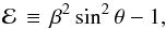 (35)which is positive
throughout this region.
(35)which is positive
throughout this region.
4.2. Near-cone divergence
Our plan is to integrate numerically two, coupled second-order equations in order to
determine the variables  and
g-2 throughout the flow. With
in hand,
another integration will yield f0 itself. Before we embark on
this program, let us consider more carefully the behavior of
and
g-2. In the upstream and downstream regions, the term
and
g-2 throughout the flow. With
in hand,
another integration will yield f0 itself. Before we embark on
this program, let us consider more carefully the behavior of
and
g-2. In the upstream and downstream regions, the term
 vanishes as one approaches either Mach cone. Thus, the source terms in Eqs. (31) and (32) diverge in that limit. Similarly, the source terms in Eqs. (33) and (34) diverge because of the vanishing of ℰ. It is possible, then, that
both and
g-2 also diverge at the cones.
vanishes as one approaches either Mach cone. Thus, the source terms in Eqs. (31) and (32) diverge in that limit. Similarly, the source terms in Eqs. (33) and (34) diverge because of the vanishing of ℰ. It is possible, then, that
both and
g-2 also diverge at the cones.
This is indeed the case. In this section, we first establish the divergences of
and
g-2 in the downstream region only. That is, we assume that
θ approaches θM from
below. Later in the section, we outline the derivation for the remaining regions of the
flow. We then use the full result to shed light on the unknown parameter
C.
Since
θ < θM, we define the positive angle
α ≡ θM − θ,
and assume that and
g-2 take the following asymptotic forms as
α diminishes:
![\begin{eqnarray} \label{eqn:fSOas} &&f_0^\prime = \zeta\,\,\alpha^{-m} \\[2.5mm] \label{eqn:gSOas} &&g_{-2} = \gamma\,\,\alpha^{-n} , \end{eqnarray}](/articles/aa/full_html/2014/01/aa22829-13/aa22829-13-eq148.png) where
ζ, γ, m, and n are
all functions of β only. If both and
g-2 truly diverge, then m and
n are positive. Within Eqs. (31) and (32), we replace
sin θ and cos θ by their limiting values,
1/β and
where
ζ, γ, m, and n are
all functions of β only. If both and
g-2 truly diverge, then m and
n are positive. Within Eqs. (31) and (32), we replace
sin θ and cos θ by their limiting values,
1/β and  , respectively. We further note
that
, respectively. We further note
that  .
After differentiating the asymptotic forms of and
g-2 with respect to θ, we derive
simplified, limiting forms of Eqs. (31)
and (32). Expressed using
α as the independent variable, these are
.
After differentiating the asymptotic forms of and
g-2 with respect to θ, we derive
simplified, limiting forms of Eqs. (31)
and (32). Expressed using
α as the independent variable, these are 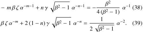 In
deriving these equations, we have retained only the most rapidly diverging terms on the
right-hand sides of Eqs. (31) and (32). We have also dropped terms proportional
to α−m and
α−n in the left-hand side of Eq. (31), since both terms are dominated, in the
small-α limit, by the two we have kept.
In
deriving these equations, we have retained only the most rapidly diverging terms on the
right-hand sides of Eqs. (31) and (32). We have also dropped terms proportional
to α−m and
α−n in the left-hand side of Eq. (31), since both terms are dominated, in the
small-α limit, by the two we have kept.
We next consider the β-dependence of m and n. The right-hand side of Eq. (39) is proportional to α-2. For this equation to balance as α diminishes, one left-hand term could also diverge as α-2, and the other more slowly. However, if this were the case, i.e., if either m = 2 > nor n = 2 > m , then Eq. (38) would be unbalanced. It is also posssible that the two left-hand terms in (39) diverge more rapidly than α-2, balancing each other. We would then have m = n > 2 . Finally, all three terms in Eq. (39) could diverge at the same rate: m = n = 2 .
Assuming provisionally that m = n > 2 , then we may ignore the right-hand terms of both Eqs. (38) and (39) in the asymptotic limit. After dividing out all terms containing α, the two equations reduce to
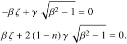 Adding
these two yields
Adding
these two yields 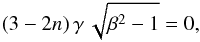 which
implies that n = 3/2 . Since we assumed
n > 2at the outset, our original hypothesis,
m = n > 2 , was incorrect.
which
implies that n = 3/2 . Since we assumed
n > 2at the outset, our original hypothesis,
m = n > 2 , was incorrect.
We have established that m = n = 2 . Equations (38) and (39) now reduce asymptotically to 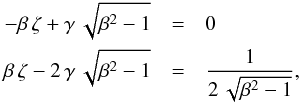 which
have the unique solution
which
have the unique solution 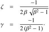 Consider
next the region just upstream from the Mach cone. Here, we may assume the same asymptotic
forms for and
g-2 as in Eqs. (36) and (37), provided the
independent variable α remains positive:
α ≡ θ − θM.
Inserting these functional forms into the second-order Eqs. (33) and (34), we note
that dα/dθ changes sign from −1 to
+1, and that ℰ now approaches
Consider
next the region just upstream from the Mach cone. Here, we may assume the same asymptotic
forms for and
g-2 as in Eqs. (36) and (37), provided the
independent variable α remains positive:
α ≡ θ − θM.
Inserting these functional forms into the second-order Eqs. (33) and (34), we note
that dα/dθ changes sign from −1 to
+1, and that ℰ now approaches  near the cone. We then derive equations analogous to (38) and (39), which
may again be solved in the near-cone limit. After applying similar reasoning to the two
regions surrounding the anti-Mach cone, we arrive at the following asymptotic forms for
and
g-2 near θM and
:
near the cone. We then derive equations analogous to (38) and (39), which
may again be solved in the near-cone limit. After applying similar reasoning to the two
regions surrounding the anti-Mach cone, we arrive at the following asymptotic forms for
and
g-2 near θM and
:
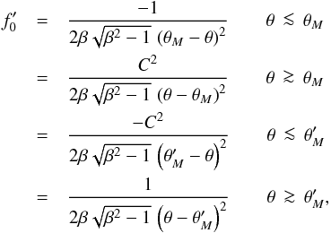 (40)and
 (41)Obtaining
f0 requires that we integrate
over
θ. Starting at the upstream axis, with
f0(π) = 0 , the integrated
f0(θ) diverges to positive infinity as
θ approaches . However, the
stream function has a direct physical meaning as the mass transfer rate into a surface of
revolution. Since this rate is finite for any θ, the function
(41)Obtaining
f0 requires that we integrate
over
θ. Starting at the upstream axis, with
f0(π) = 0 , the integrated
f0(θ) diverges to positive infinity as
θ approaches . However, the
stream function has a direct physical meaning as the mass transfer rate into a surface of
revolution. Since this rate is finite for any θ, the function
 must be integrable across the
anti-Mach cone. That is, the upward divergence of for
must be integrable across the
anti-Mach cone. That is, the upward divergence of for
 must be cancelled by
a matching downward divergence for
must be cancelled by
a matching downward divergence for  . A similar
antisymmetry of the divergences must occur at the Mach cone,
θ = θM(see Fig. 4). Inspection of Eq. (40) shows that this requirement forces C2
to be unity. The parameter C itself is either +1 or −1, independent of
β. We will demonstrate presently that the positive solution is the
physically relevant one.
. A similar
antisymmetry of the divergences must occur at the Mach cone,
θ = θM(see Fig. 4). Inspection of Eq. (40) shows that this requirement forces C2
to be unity. The parameter C itself is either +1 or −1, independent of
β. We will demonstrate presently that the positive solution is the
physically relevant one.
4.3. Vorticity
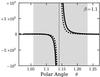 |
Fig. 4 Asymmetric divergences at the Mach angle, for β = 1.1 . The solid
and dashed curves trace |
The second-order flow must be irrotational, as we argued in Sect. 3.3. Starting with Eq. (25), we again replace the velocity components by ψ and ρ, and develop the latter in our perturbation series. Equating coefficients of r-2 tests irrotationality in the second-order flow. Specifically, we require
 (42)Within
the upstream and downstream regions, Eqs. (15) and (16) give us
f1 and g-1, respectively.
Substituting these functions into Eq. (42)
then yields the condition of irrotationality:
(42)Within
the upstream and downstream regions, Eqs. (15) and (16) give us
f1 and g-1, respectively.
Substituting these functions into Eq. (42)
then yields the condition of irrotationality: 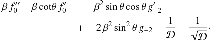 (43)Finally,
we may combine this last relation with Eq. (31), the r-component of Euler’s equation, to obtain
(43)Finally,
we may combine this last relation with Eq. (31), the r-component of Euler’s equation, to obtain
 (44)This
is identical to Eq. (I.64), and will prove useful when we evaluate the force.
(44)This
is identical to Eq. (I.64), and will prove useful when we evaluate the force.
Turning to the intermediate region, we need to use Eqs. (21) and (22) for
f1, g-1, and their derivatives.
In both equations, the unknown parameter C appears. Substitution into Eq.
(42) above yields the condition for
irrotationality: 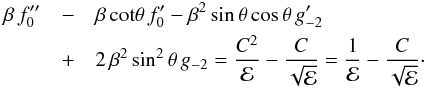 (45)In
the last form of this equation, we have used the fact that
C2 = 1 . Combination with the Euler Eq. (31) gives
(45)In
the last form of this equation, we have used the fact that
C2 = 1 . Combination with the Euler Eq. (31) gives 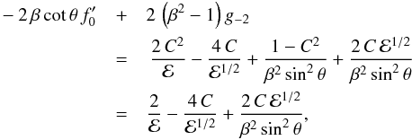 (46)which
will again aid in the force evaluation.
(46)which
will again aid in the force evaluation.
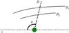 |
Fig. 5 Enforcing irrotationality. In our steady-state, isothermal flow, the Bernoulli function B is constant along each streamline. In principle, B could vary from one streamline to the next. However, if we also make B constant along any cone, then the function is a universal constant and the flow is irrotational. |
We emphasize a key difference between Eqs. (44) and (46). Because the upstream and downstream regions join smoothly onto the uniform background, the flow in both is guaranteed to be irrotational to all orders. In our numerical determination of the flow, to be described in Sect. 4.5 below, we verified that Eq. (44) indeed holds numerically both upstream and downstream. In contrast, we need to impose Eq. (46), or an equivalent condition, to obtain a physically acceptable solution in the intermediate region.
Enforcing irrotationality in the intermediate region requires only that we impose this
condition along any interior cone, i.e., at a θ-value such that
. To see
why, return to Euler’s equation, in the form given by Eq. (23). Projecting this vector equation along the
r-direction gives 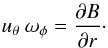 This
relation holds at fixed θ and φ. Since the flow is
axisymmetric, the equation also holds at all φ-values, i.e., along a
cone. If ωφ vanishes along such a cone, then
B is constant on that surface:
∂B/∂r = 0 . But we already know
that B does not vary along any streamline. As Fig. 5 illustrates schematically, the additional constraint tells us that the
B-values characterizing each streamline are identical, i.e.,
B is a true spatial constant. Thus,
∇B = 0and, from Eq. (23), the flow is irrotational.
This
relation holds at fixed θ and φ. Since the flow is
axisymmetric, the equation also holds at all φ-values, i.e., along a
cone. If ωφ vanishes along such a cone, then
B is constant on that surface:
∂B/∂r = 0 . But we already know
that B does not vary along any streamline. As Fig. 5 illustrates schematically, the additional constraint tells us that the
B-values characterizing each streamline are identical, i.e.,
B is a true spatial constant. Thus,
∇B = 0and, from Eq. (23), the flow is irrotational.
In practice, we apply ωφ = 0at
θ = π/2 , the equatorial plane of
the flow. The irrotationality condition, expressed as Eq. (46), implies that there is a unique (but β-dependent)
value of g-2 at that angle:  (47)When
we find the flow numerically in the intermediate region, we will impose Eq. (47) as an initial condition. The resulting
flow is then irrotational. That is, all solutions of Euler’s Eqs. (33) and (34) also obey Eq. (46).
(47)When
we find the flow numerically in the intermediate region, we will impose Eq. (47) as an initial condition. The resulting
flow is then irrotational. That is, all solutions of Euler’s Eqs. (33) and (34) also obey Eq. (46).
4.4. Mass accretion
It is only in the second-order flow that mass accretion onto the central object appears. Moreover, the function f0(θ), evaluated on the downstream axis, gives the actual accretion rate. Higher-order approximations to the flow contribute no additional information in this regard. We now review the argument, first advanced in Paper I, and apply it to the present, supersonic, case.
Consider the net transfer rate of mass into a sphere of radius r. In a
steady-state flow, this rate is the same through any closed surface; we simply use a
sphere for convenience. The dimensional result is 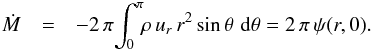 (48)Here
we have substituted Eq. (2) for
ur and utilized the normalization for the
stream function, ψ(r,π) = 0 3. We have also implicitly assumed that ρ and
ur are smooth functions, despite the
divergences arising in their perturbation expansions.
(48)Here
we have substituted Eq. (2) for
ur and utilized the normalization for the
stream function, ψ(r,π) = 0 3. We have also implicitly assumed that ρ and
ur are smooth functions, despite the
divergences arising in their perturbation expansions.
If we identify  as our
fiducial mass accretion rate, then the non-dimensional counterpart of the last equation
becomes
as our
fiducial mass accretion rate, then the non-dimensional counterpart of the last equation
becomes  Substitution
of the series expansion for ψ(r,0) in Eq. (6) and application of the boundary condition
that fi(0) = 0for
i = 1, −1, −2, etc. leads to
Substitution
of the series expansion for ψ(r,0) in Eq. (6) and application of the boundary condition
that fi(0) = 0for
i = 1, −1, −2, etc. leads to
 (49)It is noteworthy that
Ṁ depends only on a coefficient from the second-order expansion; this
fact calls for a more physical explanation. One reason is that the streamlines of the
first-order flow are symmetric, so that accretion does not occur to this approximation.
Secondly, the mass flux
ρ ur, when expanded
using approximations higher than second-order, generates terms that fall off faster than
r-2. After integrating these terms over a large bounding
sphere and taking the large-r limit, they do not contribute to
Ṁ. In any event, Eq. (49) underscores the fact that the function
must be integrable across both
Mach cones, despite its divergent behavior at the cones themselves.
(49)It is noteworthy that
Ṁ depends only on a coefficient from the second-order expansion; this
fact calls for a more physical explanation. One reason is that the streamlines of the
first-order flow are symmetric, so that accretion does not occur to this approximation.
Secondly, the mass flux
ρ ur, when expanded
using approximations higher than second-order, generates terms that fall off faster than
r-2. After integrating these terms over a large bounding
sphere and taking the large-r limit, they do not contribute to
Ṁ. In any event, Eq. (49) underscores the fact that the function
must be integrable across both
Mach cones, despite its divergent behavior at the cones themselves.
We may now use our second-order equations to obtain a useful relation between
f0(0), and hence the mass accretion rate, and the flow
density. Consider first the upstream and downstream regions. The left-hand side of Eq.
(32) is a perfect derivative:
![\begin{eqnarray*} -\beta\,f_0^\prime + {\cal D}\,g_{-2}^\prime &-& 2\,\beta^2\,{\rm sin}\,\theta\,{\rm cos}\,\theta\,g_{-2} \\ &=& {{{\rm d}\phantom r}\over{{\rm d}\theta}} \left[-\beta\,f_0 + \left(1 - \beta^2\,{\rm sin}\,\theta\right)\,g_{-2} \right]. \end{eqnarray*}](/articles/aa/full_html/2014/01/aa22829-13/aa22829-13-eq205.png) In
the right-hand side of the same equation, we note that
is an even function, in the sense that
In
the right-hand side of the same equation, we note that
is an even function, in the sense that  . Since cos θ is an odd function,
cos θ = −cos (π − θ) , the
entire right-hand side of Eq. (32) is odd.
. Since cos θ is an odd function,
cos θ = −cos (π − θ) , the
entire right-hand side of Eq. (32) is odd.
Within the intermediate region, the left-hand side of Eq. (34) is ![\begin{eqnarray*} -\beta\,f_0^\prime - {\cal E}\,g_{-2}^\prime &- & 2\,\beta^2\,{\rm sin}\,\theta\,{\rm cos}\,\theta\,g_{-2} \,\\ &=& {{{\rm d}\phantom r}\over{{\rm d}\theta}} \left[-\beta\,f_0 + \left(1 - \beta^2\,{\rm sin}^2\,\theta\right)\,g_{-2} \right] . \end{eqnarray*}](/articles/aa/full_html/2014/01/aa22829-13/aa22829-13-eq208.png) Again,
the right-hand side of Eq. (34) is odd.
Now the integral of an odd function from the downstream to the upstream axes vanishes.
Thus, if we integrate Eq. (32) from
θ = 0to θM, Eq. (34) from
θM to
, and Eq.
(32) from
to
π, we find that
Again,
the right-hand side of Eq. (34) is odd.
Now the integral of an odd function from the downstream to the upstream axes vanishes.
Thus, if we integrate Eq. (32) from
θ = 0to θM, Eq. (34) from
θM to
, and Eq.
(32) from
to
π, we find that  Using
f0(π) = 0 , we have the desired result:
Using
f0(π) = 0 , we have the desired result:
 (50)The same relation
appeared in the subsonic study as Eq. (I.46).
(50)The same relation
appeared in the subsonic study as Eq. (I.46).
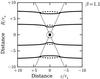 |
Fig. 6 First-order streamlines. Shown are contours of constant f2 r2 + f1 r, for the case β = 1.1 . The dotted, diagonal lines trace the Mach and anti-Mach cones, while the central, dotted circle is r/rs = 1 . Within the intermediate region, the dashed streamlines were constructed assuming C = −1 . The solid ones correspond to C = +1and are more realistic. |
4.5. Numerical solution
4.5.1. Evaluation of C
Our description of the flow is clearly incomplete until we identify the still unknown parameter C, and not just its absolute value. We again employ physical reasoning. The value of C affects the shape of the streamlines, even in the first-order flow. Only one shape is reasonable dynamically. Figure 6 shows streamlines of the first-order flow for the case β = 1.1 . That is, we plot contours of constant f2 r2 + f1 r . In the upstream and donwstream regions, f1 is taken from Eq. (15). For the intermediate region, we use Eq. (21), with both C = +1(solid curves) and C = −1(dashed curves). For either choice of the parameter, we see that all first-order streamlines are symmetric about the equatorial plane, as we found in the subsonic flow (see, e.g., Fig. I.2). The kinks at both Mach cones result from the crudeness of this first-order approximation, and would disappear in successively more accurate treatments.
The solid curves in Fig. 6 bow inward, toward the central mass, both upstream of the anti-Mach cone and inside it. Such inward turning results naturally from the gravitational pull of the mass. Eventually, the concurrent rise in density and pressure pushes the gas outward. If we were instead to choose C = −1 , the streamlines in the intermediate region would bow outward, which is not expected.
We may also consider the matter more quantitatively by examining the velocity component
uR. Here R is the
cylindrical radius:
R ≡ r sin θ . In the
far-field limit, uR tends to zero, since
the background flow is in the z-direction. Closer to the equatorial
plane, but still upstream, uR should be
slightly negative. Downstream, this velocity component should reverse sign as each
streamline rejoins the background flow. Starting with the expreessions for
f1 and g-1 in the intermediate
region, we first calculate ur and
uθ from Eqs. (2) and (3), and then obtain
uR ≡ ur sin θ + uθ cos θ
. We find that ![\begin{eqnarray*} u_R = \left[\frac{C - {\cal E}^{1/2}}{r\,\beta\,{\cal E}^{1/2}}\right] {\rm cot}\,\theta . \end{eqnarray*}](/articles/aa/full_html/2014/01/aa22829-13/aa22829-13-eq220.png) Upstream
from the mass
Upstream
from the mass  ,
we have cot θ > 0 . Thus, if
C = −1 , then
uR > 0in
this direction. Conversely,
uR < 0downstream
from the mass. This behavior is contrary to the physically reasonable one, so we
conclude that C = +1 .
,
we have cot θ > 0 . Thus, if
C = −1 , then
uR > 0in
this direction. Conversely,
uR < 0downstream
from the mass. This behavior is contrary to the physically reasonable one, so we
conclude that C = +1 .
4.5.2. Integration scheme
Determining the second-order flow requires that we numerically integrate Eqs. (31) and (32) in the upstream and downstream regions, and Eqs. (33) and (34), with C = +1 , in the intermediate region. In
all cases, we need to specify appropriate boundary values of
and
g-2. We then perform an additional integration to obtain
f0 and thereby the streamlines.
One of our boundary conditions is the value of f0(0). As we
have seen, this quantity is also the mass accretion rate Ṁ. There is
still no fundamental theory to supply this rate, except at β = 0(Bondi 1952), and in the hypersonic
(β ≫ 1)limit (Hoyle &
Lyttleton 1939; Bondi & Hoyle
1944). Extending the work of Bondi
(1952), Moeckel & Throop (2009)
suggested an interpolation formula that both respects the analytic limits and agrees
reasonably well with numerical simulations. As we did in Paper I, we adopt this
prescription, which is  (51)Here,
2 λ = e3/2/2 = 2.24is
the analytic value of Ṁ(0) in the isothermal case (Bondi 1952).
(51)Here,
2 λ = e3/2/2 = 2.24is
the analytic value of Ṁ(0) in the isothermal case (Bondi 1952).
We are now in a position to outline our numerical procedure. Starting at the upstream
axis, θ = π , we set
 . We provisionally treat
g-2(π) as a free parameter, to be
determined later in order to ensure smoothness of the flow across the Mach cones, as we
describe in more detail below. For any selected
g-2(π), we may then integrate Eqs. (31) and (32) to the anti-Mach cone,
. We provisionally treat
g-2(π) as a free parameter, to be
determined later in order to ensure smoothness of the flow across the Mach cones, as we
describe in more detail below. For any selected
g-2(π), we may then integrate Eqs. (31) and (32) to the anti-Mach cone,  .
Simultaneous integration of yields
f0 itself.
.
Simultaneous integration of yields
f0 itself.
But knowledge of both g-2(π) and
f0(0) also gives us g-2(0),
according to Eq. (50). Since
 , we may again integrate
the second-order Eqs. (31) and (32), along with
, from
θ = 0to
θ = θM . At this
point, we have established a one-parameter family of flows covering both the upstream
and downstream regions. For any value of
g-2(π), both flows are irrotational, as
required physically.
, we may again integrate
the second-order Eqs. (31) and (32), along with
, from
θ = 0to
θ = θM . At this
point, we have established a one-parameter family of flows covering both the upstream
and downstream regions. For any value of
g-2(π), both flows are irrotational, as
required physically.
Turning to the intermediate region, we begin at the equatorial plane,
θ = π/2 . We use Eq. (47) for
g-2(π/2) , again
setting C = +1 . Our free parameter is now
 . For any value of this
quantity, we integrate Eqs. (33) and
(34) away from the plane in both
directions until we come to the Mach cones. We have then established the run of
and
g-2 throughout the intermediate region. Again, the flow is
irrotational for any value of 4.
. For any value of this
quantity, we integrate Eqs. (33) and
(34) away from the plane in both
directions until we come to the Mach cones. We have then established the run of
and
g-2 throughout the intermediate region. Again, the flow is
irrotational for any value of 4.
4.5.3. Enforcing smoothness
Within the intermediate region, we only know f0 up to a
constant of integration, which has yet to be fixed. In addition, we have not yet
determined our two free parameters, and
g-2(π). All three quantities are
specified by requiring that the flow be smoothly varying. If
and
g-2 were well-defined everywhere, this task would be
straightforward. For example, we could tune one parameter until
g-2, as calculated in the downstream region, matched the
intermediate g-2 at the Mach cone. However, both
and
g-2 diverge at the cones. Hence, we can only require
smoothness outside some finite region surrounding each cone.
We therefore stopped each integration at a point where the divergent behavior begins to
dominate. For example, when integrating from θ = π ,
we examined the ratio  . Since
 , this quantity is close to
unity for θ ≲ π . However, α climbs
sharply near . In
practice, we stopped the integration at α = 10. We adopted equivalent
criteria in the other regions. thus establishing boundaries for the well-behaved flow.
Finally, we chose and
g-2(π) so that
f0 and g-2 matched as closely
as possible across these boundaries.
, this quantity is close to
unity for θ ≲ π . However, α climbs
sharply near . In
practice, we stopped the integration at α = 10. We adopted equivalent
criteria in the other regions. thus establishing boundaries for the well-behaved flow.
Finally, we chose and
g-2(π) so that
f0 and g-2 matched as closely
as possible across these boundaries.
A convenient measure of the goodness of fit is  (52)Here,
 is
difference of g-2 across the anti-Mach cone, and the two
other quantities are analogously defined. We separately enforced
is
difference of g-2 across the anti-Mach cone, and the two
other quantities are analogously defined. We separately enforced
 by adding the appropriate
constant to the numerical integration of in the
intermediate region. As we varied both and
g-2(π), the quantity χ
reached a well-defined minimum. Figure 7 shows
χ-contours for the case β = 1.1 . The optimal values
of and
g-2(π), shown here by the dot within the
circle, were insensitive to our choice of α.
by adding the appropriate
constant to the numerical integration of in the
intermediate region. As we varied both and
g-2(π), the quantity χ
reached a well-defined minimum. Figure 7 shows
χ-contours for the case β = 1.1 . The optimal values
of and
g-2(π), shown here by the dot within the
circle, were insensitive to our choice of α.
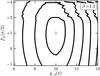 |
Fig. 7 Contours of constant χ, where χ is defined by
Eq. (52) in the text. Adjacent
contours are separated by a χ-interval of 15.0. The minimum
point, indicated by the central dot within the circle, is
|

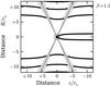 |
Fig. 8 Streamlines of the second-order flow, for β = 1.1 , constructed using the best-fit parameters from Fig. 7. The shaded regions surrounding the two Mach cones represent sectors in which the perturbation coefficients diverge. Also indicated are the central mass and the surrounding circle corresponding to r = 1 . Notice that the innermost streamlines reach the origin, indicating the occurrence of mass accretion. |
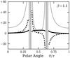 |
Fig. 9 Angular variation of perturbation coefficients for β = 1.1 . The
dashed curves show |
4.5.4. Sample results
With the numerical procedure in hand, we could determine the second-order flow for any desired β. Figure 8 displays streamlines for β = 1.1. Even in this modestly supersonic case, the two Mach cones depart substantially from the equatorial plane (θM = 65°) , and the isodensity contours are a set of nearly vertical lines that bow inward slightly toward the mass. The shaded interiors of the wedges straddling each Mach cone represent the excluded sectors within which the divergent behavior dominates. We previously indicated the excluded region surrounding the Mach cone by the shading in Fig. 4.
Returning to Fig. 8, we notice that the streamlines in the intermediate region have the expected concavity, but are not precisely symmetric across the equatorial plane. For example, a cone with a half angle of θ = 50° cuts the outermost streamlines shown at a radius that is 1% closer downstream than upstream. Notice also how the innermost streamlines join onto the central mass. The surface of revolution they generate encloses the full Ṁ, and the figure illustrates that mass accretion occurs in this order of approximation. However, we cannot obtain the detailed behavior of the flow as it joins onto the mass, since our perturbation series is only valid well outside r = 1 , the boundary indicated here as the central, dashed circle.
Figure 9 shows the angular variation of
(dashed
curve) and g-2 (dotted curve) for this same
β-value. As in Fig. 8, the
shaded regions mark those sectors where both variables diverge. By design, the
coefficients diverge antisymmetrically as either cone is approached. This behavior is
not evident in the figure, which appears to show a symmetric divergence. In more detail,
both and
g-2 first rise when approaching the Mach cone from
downstream, then reach a peak and plunge downward (recall Fig. 4). They exhibit analogous behavior upstream of the anti-Mach cone.
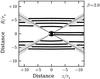 |
Fig. 10 Streamlines of the second-order flow for β = 2.0 , constructed
using |

The solid curve in Fig. 9 shows the integrated f0. The upstream and downstream values of this coefficient match exactly at the anti-Mach cone. We forced this match by adjusting the integration constant within the intermediate region. The values of f0 on either side of the Mach cone have a ratio of 1.6. This ratio depends both on our choices of f′(π/2) and g-2(π/2), and on the precise manner by which we excise the divergent region surrounding the Mach cone. Within our scheme, the mismatch is a weak function of the parameter α.
As an additional example, Fig. 10 displays streamlines of the second-order flow for β = 2.0 . Here, both cones are even more removed from the equatorial plane (θM = 30°), and the fluid elements are nearly following straight-line trajectories. The innermost pair shown here nevertheless still bends to reach the origin. Quantitatively, the fluid is affected significantly by gravity if it passes within the accretion radius racc, which varies as β-2. Notice also that the figure of revolution generated by the innermost streamlines is much narrower than in Fig. 8. This narrowing reflects the fact that Ṁ decreases steeply with β as the Mach number climbs significantly above unity.
We remind the reader that both Figs. 8 and 10 are just approximations to the actual flow. The calculated flow would become more accurate at any fixed r ≫ rs with the inclusion of higher-order terms in the perturbation series. However, the mathematical divergences at the Mach and anti-Mach cones would remain. Because of these divergences, streamlines tend to bend unphysically toward both cones. Our procedure above was designed to prevent these divergences from unduly influencing the shapes of the streamlines, at least to this order in the perturbation expansion.
5. Friction force
5.1. Integration of the momentum flux
Our reconstruction of the streamlines has a degree of arbitrariness, necessitated by the
near-cone divergence in our perturbation series. We will now show that the force
evaluation does not have this limitation, but is exact. Dimensionally, the total rate at
which z-momentum is transported into a sphere surrounding the mass is
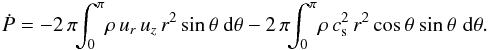 (53)The
first right-hand term is the net advection of momentum across the surface, while the
second represents the static pressure acting on the sphere. If we let our unit of force be
(53)The
first right-hand term is the net advection of momentum across the surface, while the
second represents the static pressure acting on the sphere. If we let our unit of force be
 , then the
corresponding non-dimensional expression is
, then the
corresponding non-dimensional expression is 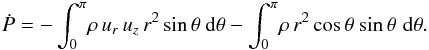 (54)The
next step is to write all velocity components in terms of ψ and
ρ, and then to expand the latter variables in their respective
perturbation series. These operations produce terms proportional to
r2, r1,
r0, etc. We are thus motivated to write
(54)The
next step is to write all velocity components in terms of ψ and
ρ, and then to expand the latter variables in their respective
perturbation series. These operations produce terms proportional to
r2, r1,
r0, etc. We are thus motivated to write 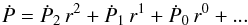 (55)Since
Ṗ is also the force on the mass, it should not depend on distance. It
is important, therefore, to check that both Ṗ2 and
Ṗ1 vanish identically. This is indeed the case. We refer the
reader to Appendix A for details of the calculation. The terms in Ṗ that
are proportional to negative powers of r diminish at large distance and
need not be calculated explicitly. For the remainder of this section, we focus on
evaluating the term Ṗ0.
(55)Since
Ṗ is also the force on the mass, it should not depend on distance. It
is important, therefore, to check that both Ṗ2 and
Ṗ1 vanish identically. This is indeed the case. We refer the
reader to Appendix A for details of the calculation. The terms in Ṗ that
are proportional to negative powers of r diminish at large distance and
need not be calculated explicitly. For the remainder of this section, we focus on
evaluating the term Ṗ0.
Results of Ruffert (1996).
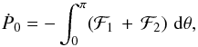
The full expression for Ṗ0 may be written as
 (56)where
 and
and
 If
we use Eqs. (15) and (16) for f1 and
g-1 in the downstream region, then we find that this
contribution to the full Ṗ0, which we label
If
we use Eqs. (15) and (16) for f1 and
g-1 in the downstream region, then we find that this
contribution to the full Ṗ0, which we label
 , is
, is
![\begin{eqnarray} \label{eqn:pdotd} {\dot P}_0^d = -\int_0^{\theta_M} \!\!{\rm d}\theta\left[\left(1-\beta^2\right) {\rm sin}\,\theta\,{\rm cos}\,\theta\,g_{-2} + \beta \left(1 + {\rm cos}^2\,\theta\right)f_0^\prime\right] . \end{eqnarray}](/articles/aa/full_html/2014/01/aa22829-13/aa22829-13-eq278.png) (57)At
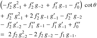
this point, we may utilize the condition of irrotationality, expressed as Eq. (44). Multiplying this latter equation by
(sin θ cos θ/2)gives
(57)At
this point, we may utilize the condition of irrotationality, expressed as Eq. (44). Multiplying this latter equation by
(sin θ cos θ/2)gives
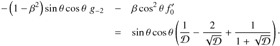 Substitution
of this last relation into Eq. (57)
transforms the latter into
Substitution
of this last relation into Eq. (57)
transforms the latter into 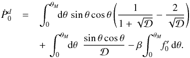 Of
the three integrals on the right-hand side, the first may be evaluated analytically, while
the second and third are divergent. After doing the first integral, we have
Of
the three integrals on the right-hand side, the first may be evaluated analytically, while
the second and third are divergent. After doing the first integral, we have 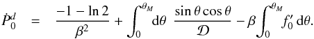 (58)Closely
analogous reasoning for the upstream contribution, to be denoted
(58)Closely
analogous reasoning for the upstream contribution, to be denoted
 , gives us
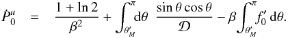 (59)For
the intermediate region, we must now use Eqs. (21) and (22) for
f1 and g-1, with
C = +1 . We find, for the contribution
(59)For
the intermediate region, we must now use Eqs. (21) and (22) for
f1 and g-1, with
C = +1 . We find, for the contribution
 , an equation
analogous to (57):
, an equation
analogous to (57): ![\begin{eqnarray} \label{eqn:pdoti} {\dot P}_0^i = -\int_{\theta_M}^{\theta_M^\prime} \!\!{\rm d}\theta\left[\left(1-\beta^2\right) {\rm sin}\,\theta\,{\rm cos}\,\theta\,g_{-2} + \beta \left(1 + {\rm cos}^2\,\theta\right)f_0^\prime\right] . \end{eqnarray}](/articles/aa/full_html/2014/01/aa22829-13/aa22829-13-eq286.png) (60)We
again avail ourselves of irrotationality, now in the form of Eq. (46). Multiplication of this last equation by
(sin θ cos θ/2)gives
(60)We
again avail ourselves of irrotationality, now in the form of Eq. (46). Multiplication of this last equation by
(sin θ cos θ/2)gives
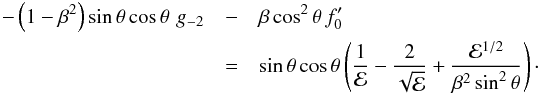 Thus,
Eq. (60) becomes
Thus,
Eq. (60) becomes 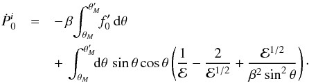 (61)The
integrand within the second right-hand term of Eq. (61) is an odd function. Since the range of integration is symmetric
about θ = π/2, this term vanishes,
and we are left with
(61)The
integrand within the second right-hand term of Eq. (61) is an odd function. Since the range of integration is symmetric
about θ = π/2, this term vanishes,
and we are left with 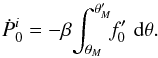 (62)Combining Eqs. (58), (59), and (62), we find
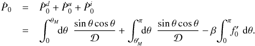 (63)Within
the second right-hand integral, let
ν ≡ π − θ . Noting that
(63)Within
the second right-hand integral, let
ν ≡ π − θ . Noting that
 , we find
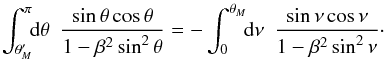 Thus,
the first and second right-hand integrals of Eq. (63) cancel, and we have
Thus,
the first and second right-hand integrals of Eq. (63) cancel, and we have 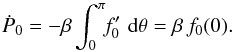 (64)Using Eq. (49), and identifying
Ṗ0 as the friction force F, we arrive at
our central result:
(64)Using Eq. (49), and identifying
Ṗ0 as the friction force F, we arrive at
our central result:  (65)Equation (65) is identical to that derived in the
subsonic case, Eq. (I.58). What we have demonstrated is that a single expression for the
force holds at all speeds. Given our assumption of a steady-state, laminar flow in the far
field, this result is exact. Although the force involves the factor Ṁ,
our expression holds even for a porous, non-accreting object, such as a globular cluster
traversing a galactic halo. The result also applies to a mass that is expelling its own
gas, e.g., a wind-emitting star. In that case, the wind can only penetrate a limited
distance before it shocks against the background flow. The dynamical friction force then
acts on both the mass and its trapped wind. Our only requirement is that the background
gas well outside of rs be undisturbed.
(65)Equation (65) is identical to that derived in the
subsonic case, Eq. (I.58). What we have demonstrated is that a single expression for the
force holds at all speeds. Given our assumption of a steady-state, laminar flow in the far
field, this result is exact. Although the force involves the factor Ṁ,
our expression holds even for a porous, non-accreting object, such as a globular cluster
traversing a galactic halo. The result also applies to a mass that is expelling its own
gas, e.g., a wind-emitting star. In that case, the wind can only penetrate a limited
distance before it shocks against the background flow. The dynamical friction force then
acts on both the mass and its trapped wind. Our only requirement is that the background
gas well outside of rs be undisturbed.
This last stipulation is overly conservative. Mathematical convenience originally motivated our choice of rs as the characteristic length scale. For supersonic flows, however, streamlines deviate from the background not inside rs, but instead inside racc ~ rs/β2 < rs. Numerical simulations show this effect (e.g., Shima et al. 1985; Ruffert 1996; Lee et al. 2013). In conclusion, it is the flow outside of racc that physically determines the force, regardless of the domain of validity for our perturbation series.
For computational purposes, we may use in Eq. (65) the interpolation formula for Ṁ given in Eq. (51): 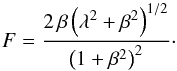 (66)We plot this relation in
Fig. 11. We also show, for comparison, the friction
force derived by Ostriker (1999), as given in her
Eqs. (14) and (15). For β > 1 , her analytic
formula includes the factor
α° ≡ ln (Vt/R),
where t is the time since the gravitational force is switched on. In the
figure, we have set α° = 2 . Notice that Ostriker’s force
diverges at β = 1 , while ours is continuous at all Mach numbers.
(66)We plot this relation in
Fig. 11. We also show, for comparison, the friction
force derived by Ostriker (1999), as given in her
Eqs. (14) and (15). For β > 1 , her analytic
formula includes the factor
α° ≡ ln (Vt/R),
where t is the time since the gravitational force is switched on. In the
figure, we have set α° = 2 . Notice that Ostriker’s force
diverges at β = 1 , while ours is continuous at all Mach numbers.
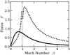 |
Fig. 11 The dynamical friction force F, shown as a function of the Mach number β. Our calculated force, taken from Eq. (66), incorporates the prescription for Ṁ from Moeckel & Throop (2009). The dotted vertical line marks β = 1 . Also shown by the broken dashed curve is the force as calculated by Ostriker (1999). This force diverges at β = 1 . |
5.2. Comparison with simulations
The numerical simulation of gas streaming past a stationary, gravitating mass has a long history. In an early work, Hunt (1971) investigated a fluid with an adiabatic index of γ = 5/3 , and with incident Mach numbers ranging from 0.6 to 2.4. A study more directly relevant to ours is that of Shima et al. (1985), whose suite of axisymmetric simulations included a γ = 1.1gas with Mach numbers again up to 2.4. The authors calculated both contributions to the friction force F – the gravitational tug from the wake, determined by integration over the density around the mass, and the advection of linear momentum through the surface of this body, a force variously called the aerodynamic or hydrodynamic drag. Despite the nomenclature, they found that this second contribution is actually a forward thrust, directed oppositely to the gravitational force. Recall that external gas does not impact the mass directly, but misses it and enters from downstream, thus imparting momentum in the upstream direction.
The total force found by Shima et al. (1985) is
greater than ours. These authors define a drag coefficient cd
through the relation
F = 2 π cd ρ0 G2 M2/V2and
an effective accretion radius reff through
 . It follows that
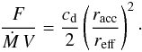 Using
their Table 1 and Fig. 9, we infer that, for
β = 0.6 , 1.4, and 2.4,
F/Ṁ V = 1.0 ,
2.4, and 3.6, respectively. Note that the radius R of their accreting
object varied with Mach number. It was set to 0.1 times racc,
so that
R = 0.2 rs/β2
.
Using
their Table 1 and Fig. 9, we infer that, for
β = 0.6 , 1.4, and 2.4,
F/Ṁ V = 1.0 ,
2.4, and 3.6, respectively. Note that the radius R of their accreting
object varied with Mach number. It was set to 0.1 times racc,
so that
R = 0.2 rs/β2
.
In a later study, Sánchez-Salcedo & Brandenburg (1999) simulated the flow of an isothermal gas around a mass whose physical size R excceds racc by a factor of 20 or more. Under these conditions, the density enhancement in the wake is relatively mild. Sánchez-Salcedo & Brandenburg (1999) switched on the gravity from the central mass suddenly, as in the calculation of Ostriker (1999). They found that their computed gravitational portion of the force closely matched Ostriker’s analytical prediction. More recently, Kim & Kim (2009), who adopted γ = 5/3, showed that this contribution to the force declines when R falls well below racc (see their Fig. 14).
The most thorough numerical investigation of the flow pattern, mass accretion rate, and
friction force for the isothermal case has been that of Ruffert (1996). In this three-dimensional simulation of a
γ = 1.01gas, both the accretor size and Mach number were varied, the
latter up to β = 10 . A general result, which corroborated and extended
those of previous studies, was that the downstream region exhibited continuing instability
for relatively small masses  embedded
in supersonic flow. These, of course, are just the conditions of most interest for our
purposes. Ruffert (1996) reported time-averaged
results for both Ṁ and F in such cases.
embedded
in supersonic flow. These, of course, are just the conditions of most interest for our
purposes. Ruffert (1996) reported time-averaged
results for both Ṁ and F in such cases.
Table 1 displays the essential results found by Ruffert (1996), both for his subsonic simulations (β = 0.6)and supersonic ones. We have only taken data from the runs in which the central mass was the smallest size. Here, the radius was 0.02 times racc. We see that, even for β = 0.6, R is less than rs, as our own study assumes. In addition to β, other non-dimensional quantities shown in the table include: Ṁ, the mass accretion rate; Ṗgrav, the gravitational contribution to the force; Ṗadv, the advective component; and their sum Ṗtot, which is also the force F. Notice that Ṗtot is positive, i.e., it points in the +z-direction in Fig. 2. The quantity Ṗadv is negative in all cases, and smaller in magnitude than Ṗtot, so that the net force indeed retards the motion of the mass relative to the background gas.
As the seventh column of the table shows, Ṗtot is not equal to Ṁ β. Even for β ~ 1 , the ratio Ṗtot/Ṁ βexceeds unity, and inreases with β, as found earlier by Shima et al. (1985). If there is no error in our theoretical derivation, what could be the source of this discrepancy?
A successful simulation must replicate the flow well in inside of racc. This task becomes more demanding at higher β, since racc itself varies as β-2. Following how the gas joins onto the central object is especially critical. Suppose, for example, that the velocity of material just outside the gravitating mass were, for any reason, artificially low in a simulation. Then, for a given Ṁ, mass conservation dictates that the density close to the object be increased. Also increased would be the value of Ṗgrav, which is obtained by integrating over the surrounding density. Conversely, Ṗadv would be decreased, since it is proportional to the angle-averaged incoming speed. Both factors would cause the numerically determined Ṗtot to be too large.
Only a modest lowering of the speed creates a significant rise in
Ṗtot. To illustrate the point, we correct for this effect by
lowering the numerically calculated Ṗgrav at each
β-value by a factor f, where
f > 1 . Simultaneously, we let
Ṗadv be increased by the same factor. There is some value of
f such that Ṗtot equals
Ṁ β: 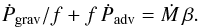 This
special f-value is listed in the last column of Table 1. As β increases by almost a factor
of 20, f is always close to unity and varies only from 1.2 to 1.3. Thus,
relatively small errors in the two force contributions, if they are inversely related,
make a big difference in Ṗtot.
This
special f-value is listed in the last column of Table 1. As β increases by almost a factor
of 20, f is always close to unity and varies only from 1.2 to 1.3. Thus,
relatively small errors in the two force contributions, if they are inversely related,
make a big difference in Ṗtot.
In an earlier paper outlining his numerical method, Ruffert (1994) stated that he softened the gravitational potential of the central mass specifically to keep the incoming velocity relatively low and thereby lengthen the computational time step (see his Sect. 2.4). Needless to say, a softened potential indeed creates such an effective deceleration. So does numerical viscosity. In the Piecewise Parabolic code that Ruffert (1994) employed, the viscosity in a region spanned by N zones scales as N-3 (Porter & Woodward 1994, p. 319). For all his isothermal simulations, Ruffert (1996) used a relatively coarse grid surrounding the mass, which typically had five zones covering a distance outside the object equal to its radius.
Since the work of Ruffert (1996), other researchers have tackled this flow problem with improved codes. Results have evolved substantially. From Table 1, Ruffert (1996) found Ṁ = 0.994for β = 1.4 . In comparison, Eq. (51), which is a fit from Moeckel & Throop (2009) to their own simulations, gives Ṁ = 0.409for the same β-value. A fresh determination of the force, using modern numerical techniques, would clearly be of interest.
We stress that both Ṁ and Ṗtot at each β should not only be calculated in the vicinity of the central mass, but also through a far-field integration. Agreement of the results obtained by these two methods would, of course, strongly corroborate the accuracy of the simulation, and also be a sensitive test that the flow has indeed reached steady state5.
5.3. Applications of the new force law
For illustrative purposes, we first consider the deceleration of a gravitating mass
traveling through a uniform gas, and subject only to the force of dynamical friction.
While the mass moves, it simultaneously accretes gas. The force is the rate of change of
the object’s momentum, so that we have the dimensional relation
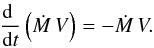 Expansion
of the derivative and integration yields
Expansion
of the derivative and integration yields  (67)where
V0 and M0 are, respectively, the
object’s initial speed and mass. We previously derived this result in Sect. 4 of Paper I.
(67)where
V0 and M0 are, respectively, the
object’s initial speed and mass. We previously derived this result in Sect. 4 of Paper I.
Pursuing the same reasoning as before, we use Ṁ from Eq. (51) to derive the non-dimensional equation
governing the velocity evolution: 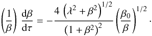 (68)Here
β0 is the initial speed, and
τ ≡ t/t0a
non-dimensional time. We have used as our fiducial dimensional time
(68)Here
β0 is the initial speed, and
τ ≡ t/t0a
non-dimensional time. We have used as our fiducial dimensional time
 (69)Here the denominator is
the fiducial mass accretion rate from Sect. 4.4. Thus, the quantity
t0 is a characteristic growth time for the mass when
β ≲ 1 , but departs from that time in the supersonic case.
(69)Here the denominator is
the fiducial mass accretion rate from Sect. 4.4. Thus, the quantity
t0 is a characteristic growth time for the mass when
β ≲ 1 , but departs from that time in the supersonic case.
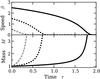 |
Fig. 12 Evolution of the particle’s speed and mass as a function of non-dimensional time τ. Mass is shown relative to its initial value. The different curves represent different initial speeds: β0 = 0.5, 1.5, and 2.5. Once the speed of an initially supersonic particle approaches β ~ 1 , it quickly decelerates. Concurrently, its mass grows rapidly. |
The upper and lower panels of Fig. 12 show the evolution of the velocity and mass, respectively, for various β0-values. Here we obtained the mass using Eq. (67). The figure includes one subsonic case, β0 = 0.5 . Notice that, when the mass starts out at supersonic speed, it first decelerates gradually, then much more sharply as β nears unity. Concurrently, its mass climbs rapidly, ultimately increasing at the Bondi rate appropriate for a stationary particle.
Turning to more concrete astrophysical applications, the frictional force may play an important role in the dynamical evolution of planets. In a relatively large fraction of exoplanets discovered through radial velocity studies, the normal to the orbital plane is misaligned with the stellar spin axis (Albrecht et al. 2012). Recently, Teyssandier et al. (2013) have simulated the evolution of an inclined, eccentric planet at the early epoch when a circumstellar disk is still present. As the planet plunges through the disk periodically, it experiences an impulsive frictional drag that gradually decreases both its orbital inclination and eccentricity, leading eventually to a coplanar, circular orbit.
In their numerical study, Teyssandier et al. (2013) found that planets with the mass of Neptune or lower can maintain their orbital inclination over the disk lifetime. On the other hand, Jovian and higher-mass planets cannot, as a result of the increased dynamical friction experienced during each disk crossing. The critical mass separating these two regimes must depend on the prescription for the frictional drag.
Teyssandier et al. (2013) used, for this drag,
both that arising from direct impact with the gas and the hypersonic limit of the force
derived by Ostriker (1999). In our non-dimensional
units, their adopted dynamical friction force
FT is  where
the factor ℐ is
where
the factor ℐ is 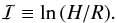 Here,
R is the radius of the planet and H is the disk’s
semi-thickness, which they used in place of Ostriker’s term
V t. The ratio of our derived force
F to this one is
Here,
R is the radius of the planet and H is the disk’s
semi-thickness, which they used in place of Ostriker’s term
V t. The ratio of our derived force
F to this one is 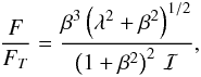 which
approaches ℐ-1 for β ≫ 1 . In their Sect. 2.4, Teyssandier et al. (2013) quote a characteristic value
of ℐ ≈ 6 . Adoption of the new, diminished friction force could significantly influence
the alignment of orbital planes, and thus the fraction of misaligned planets that survive
the disk era.
which
approaches ℐ-1 for β ≫ 1 . In their Sect. 2.4, Teyssandier et al. (2013) quote a characteristic value
of ℐ ≈ 6 . Adoption of the new, diminished friction force could significantly influence
the alignment of orbital planes, and thus the fraction of misaligned planets that survive
the disk era.
On vastly larger scales, dynamical friction also plays a role in the assembly of supermassive black holes. Accretion onto these 109 M⊙ objects powers the bright quasars detected at redshifts of z ~ 6, i.e., about 1 Gyr after the Big Bang. The most popular hypothesis is that supermassive black holes arise through the merger of “seed” black holes (M ~ 102 M⊙), which are in turn the remnants of the first stellar generation (Heger et al. 2003). The mergers occur within the dark matter haloes of coalescing galaxies. An individual black hole also accretes gas that has settled toward the center of its parent halo.
In a combined semi-analytic and numerical study, Tanaka
& Haiman (2009) showed that seed black holes can indeed form a
supermassive one in the requsite time, provided they remain embedded in the halo’s gas
component. Mass buildup is delayed by the large recoil velocities in the coalesced product
of each black hole merger. (Asymmetric gravitation radiation carries off the remaining
momentum.) Promoting the merger process is dynamical friction, which can return far-flung
black holes to the halo center. For their detailed numerical simulations, Tanaka & Haiman (2009) assumed the total
friction force to be 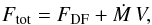 where
Ṁ is the mass accretion rate of surrounding gas. They took the
dynamical friction force FDF to be the sum of that due to the
collisionless sea of dark matter and that created by the gas. For the latter, Tanaka & Haiman (2009) adopted the formula of
Ostriker (1999).
where
Ṁ is the mass accretion rate of surrounding gas. They took the
dynamical friction force FDF to be the sum of that due to the
collisionless sea of dark matter and that created by the gas. For the latter, Tanaka & Haiman (2009) adopted the formula of
Ostriker (1999).
According to our own study, the last term above encompasses the entire gaseous dynamical friction. That is, the dynamical friction force assumed in the simulations is too large in magnitude. A diminished Ftot would increase the frequency of black hole ejections, as well as the time over which black holes flung outward remain on their extended orbits. In summary, the growth of supermassive black holes is delayed. As in the planetary problem, a revised calculation incorporating the corrected dynamical friction would be of interest.
6. Discussion
Two key assumptions underlie our derivation, and we reiterate these as a cautionary note.
The first is that the geometric size of the gravitating mass be appropriately small.
Specifically, we assume that R ≪ racc. In the
opposite extreme, R ≫ racc, the main force
acting on the object is not gravitational in origin, but comes from the direct impact of
surrounding gas. This impact force is given dimensionally by
Fimp ≈ πρ0R2V2.
The ratio of this force to that of dynamical friction is
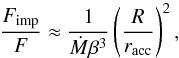 (70)where
Ṁ is non-dimensional. According to Eq. (51), the product
Ṁβ3 approaches a constant for
β ≫ 1.
(70)where
Ṁ is non-dimensional. According to Eq. (51), the product
Ṁβ3 approaches a constant for
β ≫ 1.
Our second assumption is that the gas surrounding the object be sufficiently rarefied that its self-gravity is negligible. Once the amount of mass within the radius racc becomes comparable to or exceeds that of the central object, the problem becomes one of gravitational collapse. Here, accretion generally does not occur in a steady-state manner (see also Sect. 5 of Lee et al. 2013).
The present dynamical friction calculation differs sharply both in approach and result from previous efforts. Starting with Bondi & Hoyle (1944), all other researchers have obtained expressions for the force that contain a Coulomb logarithm. This term arises from integrating over the perturbed gas, usually in the downstream wake (Bondi & Hoyle 1944; Ostriker 1999). Dokuchaev (1964) also obtained this term, but by integrating the acoustic energy flux over a large sphere surrounding the gravitating mass. His derivation is thus closer in spirit to ours. However, we are dubious of his basic premise that the total energy loss associated with the moving mass is fully accounted for by this outgoing, acoustic disturbance. Accretion generates shocks close to the mass, and the power from radiating shocks could in principle rival the acoustic loss, for a sufficiently high velocity. On the other hand, the total inflow of linear momentum is always transported unaltered to the object itself, provided the surrounding flow is steady-state.
The strategy we adopted was to use a spherical coordinate system and expand the far-field perturbations of the stream function and density in power series in the radius r. We found that various coefficients in these series diverged at both the Mach and anti-Mach cones. Since the series themselves are only valid far from the gravitating mass, these divergences are purely mathematical, and result from the specific form of the perturbation series. It may be, therefore, that all divergences could be eliminated through an appropriate change of independent variables. We leave this technical issue as a topic of future study.
Turning to our specific result, we find it compelling that the friction force in the present, supersonic case is identical in form to that found in Paper I for objects moving subsonically. Our final expression is, in fact, so simple that it raises the question of whether the complex machinery we brought to bear was necessary for its derivation. As one alternative path, consider the fact that the velocity V is the momentum per unit mass carried by the background gas. Multiplying V by Ṁ, the mass accreted per time, immediately yields the rate of momentum input, which is the force.
This concise derivation is intuitively appealing, but is also incorrect. While V is the limiting velocity of background gas at infinite distance from the mass, the true velocity differs at any finite r. Similarly, the true density differs from its background value. These differences are relatively small, but they are integrated over a large surface to obtain the net inflow of momentum. As may be seen in Sect. 5.1, this inflow is Ṁ V plus several correction terms of comparable magnitude. These additional terms cancel exactly, by virtue of the fact that the flow is irrotational. A more explicit demonstration of the analogous, subsonic result is in Sect. 5.2 of Paper I.
In any event, we do agree that a simpler derivation of our result should exist, provided the far-field flow is irrotational. Equivalently, the generalized derivation must apply to barytropic fluids, i.e., those in which P is a function only of ρ. In support of this contention, we note that Khajenabi & Dib (2012) utilized our technique of far-field integration to show that F = Ṁ Vholds for an object moving subsonically through an isentropic fluid with arbitrary adiabatic index γ. We expect that analogous reasoning will yield the same result for an isentropic fluid in the supersonic regime. At that point, the stage will be set for the new derivation, one that avoids a detailed description of the far-field flow. Whether one will still need to assume a steady-state mass accretion rate, as we have done, or be able to derive this rate from first principles, remains to be seen.
Online material
Appendix A: Background and first-order contributions to the momentum influx
Here we evaluate Ṗ2 and Ṗ1, the
first two coefficients on the right-hand side of Eq. (55). We will show that both coefficients are zero. The first is
![\appendix \setcounter{section}{1} \begin{equation} {\dot P}_2 = -\int_0^\pi \left[\left(f_2^\prime\right)^2 {\rm cot}\,\theta + 2\,f_2\,f_2^\prime + {\rm cos}\,\theta\,\,{\rm sin}\,\theta\right] {\rm d}\theta . \end{equation}](/articles/aa/full_html/2014/01/aa22829-13/aa22829-13-eq366.png) (A.1)Substituting
f2 = β sin θ/2
, this becomes
(A.1)Substituting
f2 = β sin θ/2
, this becomes 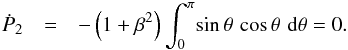 The
background flow, while it certainly carries z-momentum, makes no net
contribution to the influx.
The
background flow, while it certainly carries z-momentum, makes no net
contribution to the influx.
The integral expression for the second coefficient is lengthier, and we write it as
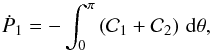 (A.2)where
 and
and
 It
is convenient to split up the integral in Eq. (A.2) by region. For the downstream part, which we denote as
It
is convenient to split up the integral in Eq. (A.2) by region. For the downstream part, which we denote as
 , we use
Eqs. (15) and (16) for f1 and
g-1. We find, after algebraic simplification, that
, we use
Eqs. (15) and (16) for f1 and
g-1. We find, after algebraic simplification, that
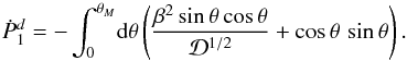 (A.3)We now use the identity
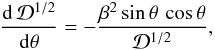
to conclude that 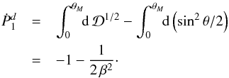 (A.4)Similarly,
the upstream part is
(A.4)Similarly,
the upstream part is 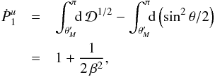 (A.5)so
that
(A.5)so
that  (A.6)For the intermediate
piece, to be denoted
(A.6)For the intermediate
piece, to be denoted  , we use
Eqs. (21) and (22) for f1 and
g-1. Although we have established that
C = +1 , we will see that is independent of
this parameter, so we retain the original notation. After algebraic manipulation, we
find
, we use
Eqs. (21) and (22) for f1 and
g-1. Although we have established that
C = +1 , we will see that is independent of
this parameter, so we retain the original notation. After algebraic manipulation, we
find 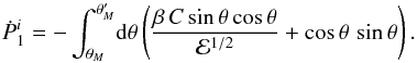 (A.7)Using the identity
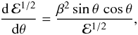 we
infer that
we
infer that 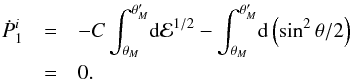 (A.8)In
summary, we have
(A.8)In
summary, we have 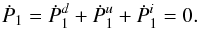 (A.9)
(A.9)
Rephaeli & Salpeter (1980) argued, based on a linear perturbation analysis, that the subsonic force vanishes. We showed in Paper I that extension of their analysis into the non-linear regime gives a finite result.
The perturbation series in Eqs. (4) and (5) are valid for r ≫ rs. On the other hand, we expect that a smooth flow, representing a modest perturbation of the background stream, is present beyond racc, which is much less than rs in the hypersonic regime. We also expect our final expression for the force to be valid as long as the background gas extends beyond racc.
On a related issue, not only do the flows in all regions have spatially uniform values of the Bernoulli function B, but these values match: B = β2/2 . To see this, we may expand Eq. (24) for B, using our perturbation series. The lowest-order (r-independent) terms sum to β2/2 in all regions, while the higher-order terms sum to zero.
Canto et al (2011) ran a simulation for β = 5 and performed a surface integration of the momentum flux over a large sphere. However, they considered only the kinetic part of the flux, i.e., the first right-hand term in our Eq.(53). The second term, from thermal pressure, is of comparable magnitude.
Acknowledgments
We thank Max Ruffert for a thoughtful referee report that helped to improve the clarity of the paper. Throughout this project, A.T.L. was supported by an NSF Graduate Fellowship, while S.W.S. received partial funding from NSF Grant 0908573.
References
- Albrecht, S., Winn, J. N., Johnson, J. A., et al. 2012, ApJ, 757, 18 [NASA ADS] [CrossRef] [Google Scholar]
- Armitage, P. J., & Natarajan, P., 2005, ApJ, 634, 921 [NASA ADS] [CrossRef] [Google Scholar]
- Bondi, H. 1952, MNRAS, 112, 195 [NASA ADS] [CrossRef] [MathSciNet] [Google Scholar]
- Bondi, H., & Hoyle, F. 1944, MNRAS, 104, 273 [NASA ADS] [CrossRef] [Google Scholar]
- Cantó, J., Raga, A. C., Esquivel, A., & Sánchez-Salcedo, F. J. 2011, MNRAS, 418, 1238 [NASA ADS] [CrossRef] [Google Scholar]
- Chandrasekhar, S. 1943, ApJ, 97, 255 [NASA ADS] [CrossRef] [Google Scholar]
- Chavarría, L., Mardones, D., Garay, G., et al. 2010, ApJ, 710, 583 [NASA ADS] [CrossRef] [Google Scholar]
- Dodd, K. N., & McCrea, W. J. 1952, MNRAS, 112, 205 [NASA ADS] [Google Scholar]
- Dokuchaev, V. P. 1964, Sov. Astron., 8, 23 [NASA ADS] [Google Scholar]
- El-Zant, A. A., Kim, W.-T., & Kamionkowski, M. 2004, MNRAS, 354, 169 [NASA ADS] [CrossRef] [Google Scholar]
- Heger, A., Fryer, C. L., Woosley, S. E., Langer, N., & Hartmann, D. H. 2003, ApJ, 591, 288 [NASA ADS] [CrossRef] [Google Scholar]
- Hoyle, F. & Lyttleton, R. A. 1939, Proc. Cambridge Philos. Soc., 35, 405 [Google Scholar]
- Hunt, R. 1971, MNRAS, 154, 141 [NASA ADS] [Google Scholar]
- Khajenab, F., & Dib, S. 2012, Ap&SS, 340, 117 [NASA ADS] [CrossRef] [Google Scholar]
- Kim, H., & Kim, W.-T. 2009, ApJ, 703, 1278 [NASA ADS] [CrossRef] [Google Scholar]
- Lee, A. T., & Stahler, S. W. 2011, MNRAS, 416, 3177 (Paper I) [NASA ADS] [CrossRef] [Google Scholar]
- Lee, A. T., Cunningham, A. J., Mckee, C. F., & Klein, R. I. 2013, ApJ, submitted [Google Scholar]
- Matsuda, T., Inoue, M., & Sawada, K. 1987, MNRAS, 226, 785 [NASA ADS] [CrossRef] [Google Scholar]
- Moeckel, N., & Throop, H. B. 2009, ApJ, 707, 269 [Google Scholar]
- Narayan, R. 2000, ApJ, 536, 663 [NASA ADS] [CrossRef] [Google Scholar]
- Ostriker, E. 1999, ApJ, 513, 252 [NASA ADS] [CrossRef] [Google Scholar]
- Pogorelov, N. V., Ohsugi, Y., & Matsuda, T. 2000, MNRAS, 313, 198 [NASA ADS] [CrossRef] [Google Scholar]
- Porter, D. H., & Woodward, P. R. 1994, ApJS, 93, 209 [Google Scholar]
- Rephaeli, Y., & Salpeter, E. E. 1980, ApJ, 240, 20 [NASA ADS] [CrossRef] [Google Scholar]
- Ricker, P. M., & Taam, R. E. 2008, ApJ, 672, L41 [NASA ADS] [CrossRef] [Google Scholar]
- Ruderman, M. A., & Spiegel, E. A. 1971, ApJ, 165, 1 [NASA ADS] [CrossRef] [Google Scholar]
- Ruffert, M. 1994, A&AS, 106, 505 [NASA ADS] [Google Scholar]
- Ruffert, M. 1996, A&A, 311, 817 [NASA ADS] [Google Scholar]
- Sánchez-Salcedo, F. J., & Brandenburg, A. 1999, ApJ, 522, L35 [NASA ADS] [CrossRef] [Google Scholar]
- Shima, E., Matsuda, T., Takeda, H., & Sawada, K. 1985, MNRAS, 217, 367 [NASA ADS] [Google Scholar]
- Tanaka, T., & Haiman, Z. 2009, ApJ, 696, 1798 [NASA ADS] [CrossRef] [Google Scholar]
- Teyssandier, J., Terquem, C., & Papaloizou, J. 2013, MNRAS, 428, 658 [NASA ADS] [CrossRef] [Google Scholar]
- Zel’dovich, Ya. B., & Raizer, Yu. P. 1968, Physics of Shock Waves and High-Temperature Hydrodynamic Phenomena (New York: Academic Press), I [Google Scholar]
All Tables
All Figures
|
Fig. 1 Sketch of mass and momentum flow. Surrounding the central gravitating body of mass M is a large, imaginary sphere. The thin curves represent streamlines of background gas. After entering the sphere, most gas simply exits again, while a small portion joins directly onto the mass. In addition, some gas temporarily forms an overdense wake, also sketched here. The wake tugs gravitationally on the mass, thereby imparting momentum to it (broad arrow). All gas entering the wake also leaves it, either joining the mass or exiting the sphere. |
| In the text | |
|
Fig. 2 Mathematical treatment of the flow. We erect a spherical coordinate system centered
on the gravitating body. The gas is isothermal, and its velocity far upstream is
β cs (β > 1).
Indicated are the Mach angle θM and its
supplement, |
| In the text | |
|
Fig. 3 Regions of the flow. The upstream and downstream regions lie within the anti-Mach and Mach cones, respectively. Between the two cones is the intermediate region. In the far-field flow, there are no physical barriers between the intermediate region and its neighbors, although mathematical divergences appear at the two cones. |
| In the text | |
|
Fig. 4 Asymmetric divergences at the Mach angle, for β = 1.1 . The solid
and dashed curves trace |
| In the text | |
|
Fig. 5 Enforcing irrotationality. In our steady-state, isothermal flow, the Bernoulli function B is constant along each streamline. In principle, B could vary from one streamline to the next. However, if we also make B constant along any cone, then the function is a universal constant and the flow is irrotational. |
| In the text | |
|
Fig. 6 First-order streamlines. Shown are contours of constant f2 r2 + f1 r, for the case β = 1.1 . The dotted, diagonal lines trace the Mach and anti-Mach cones, while the central, dotted circle is r/rs = 1 . Within the intermediate region, the dashed streamlines were constructed assuming C = −1 . The solid ones correspond to C = +1and are more realistic. |
| In the text | |
|
Fig. 7 Contours of constant χ, where χ is defined by
Eq. (52) in the text. Adjacent
contours are separated by a χ-interval of 15.0. The minimum
point, indicated by the central dot within the circle, is
|
| In the text | |
|
Fig. 8 Streamlines of the second-order flow, for β = 1.1 , constructed using the best-fit parameters from Fig. 7. The shaded regions surrounding the two Mach cones represent sectors in which the perturbation coefficients diverge. Also indicated are the central mass and the surrounding circle corresponding to r = 1 . Notice that the innermost streamlines reach the origin, indicating the occurrence of mass accretion. |
| In the text | |
|
Fig. 9 Angular variation of perturbation coefficients for β = 1.1 . The
dashed curves show |
| In the text | |
|
Fig. 10 Streamlines of the second-order flow for β = 2.0 , constructed
using |
| In the text | |
|
Fig. 11 The dynamical friction force F, shown as a function of the Mach number β. Our calculated force, taken from Eq. (66), incorporates the prescription for Ṁ from Moeckel & Throop (2009). The dotted vertical line marks β = 1 . Also shown by the broken dashed curve is the force as calculated by Ostriker (1999). This force diverges at β = 1 . |
| In the text | |
|
Fig. 12 Evolution of the particle’s speed and mass as a function of non-dimensional time τ. Mass is shown relative to its initial value. The different curves represent different initial speeds: β0 = 0.5, 1.5, and 2.5. Once the speed of an initially supersonic particle approaches β ~ 1 , it quickly decelerates. Concurrently, its mass grows rapidly. |
| In the text | |
Current usage metrics show cumulative count of Article Views (full-text article views including HTML views, PDF and ePub downloads, according to the available data) and Abstracts Views on Vision4Press platform.
Data correspond to usage on the plateform after 2015. The current usage metrics is available 48-96 hours after online publication and is updated daily on week days.
Initial download of the metrics may take a while.