| Issue |
A&A
Volume 555, July 2013
|
|
|---|---|---|
| Article Number | A117 | |
| Number of page(s) | 13 | |
| Section | Cosmology (including clusters of galaxies) | |
| DOI | https://doi.org/10.1051/0004-6361/201321215 | |
| Published online | 10 July 2013 | |
Cosmic radio dipole from NVSS and WENSS
Fakultät für Physik, Universität Bielefeld,
Postfach 100131,
33501
Bielefeld,
Germany
e-mail:
matthiasr@physik.uni-bielefeld.de; dschwarz@physik.uni-bielefeld.de
Received:
1
February
2013
Accepted:
30
May
2013
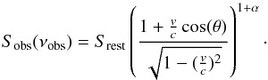
We use linear estimators to determine the magnitude and direction of the cosmic radio dipole from the NRAO VLA Sky Survey (NVSS) and the Westerbork Northern Sky Survey (WENSS). We show that special attention has to be given to the issues of bias due to shot noise, incomplete sky coverage and masking of the Milky Way. We compare several different estimators and show that conflicting claims in the literature can be attributed to the use of different estimators. We find that the NVSS and WENSS estimates of the cosmic radio dipole are consistent with each other and with the direction of the cosmic microwave background (CMB) dipole. We find from the NVSS a dipole amplitude of (1.8 ± 0.6) × 10-2 in direction (RA,dec) = (154° ± 19°, −2° ± 19°). This amplitude exceeds the one expected from the CMB by a factor of about 4 and is inconsistent with the assumption of a pure kinetic origin of the radio dipole at 99.6% CL.
Key words: radio continuum: galaxies / large-scale structure of Universe
© ESO, 2013
1. Introduction
The assumed isotropy and homogeneity of the Universe at large scales is fundamental to modern cosmology. The isotropy is best seen in the cosmic microwave background (CMB) radiation and holds at the per cent level. The most prominent anisotropy of the CMB temperature is a dipole signal of ΔT/ T ≈ 10-3. It is commonly assumed that this dipole is largely caused by the motion of the Solar system through the Universe (Stewart & Sciama 1967). This interpretation seems to be fully consistent with the concordance model of cosmology.
However, the observation of the microwave sky is not enough to tell the difference between
a motion induced CMB dipole and dipole contributions form other physical phenomena, i.e.
 (1)In our notation a
dipole vector d modulates the isotropic sky by a factor
(1)In our notation a
dipole vector d modulates the isotropic sky by a factor
 ,
with
,
with  denoting the position on the sky.
Usually it is assumed that the primordial and the integrated Sachs-Wolfe (ISW) contribution to the CMB dipole are negligibly small and that foregrounds (the Milky Way) are under control. Within the concordance model we expect a primordial contribution of dprimordial ≈ 2 × 10⁻⁵. The ISW contribution could be as large as 10-4 from the gravitational potentials induced by local 100 Mpc sized structures, without being in conflict with the concordance model (Rakic et al. 2006; Francis & Peacock 2010). The noise term can be ignored due to excellent statistics of full sky observations. Thus the measured dcmb is directly used to infer the velocity of the Solar system w.r.t. the CMB to be v = 369 ± 0.9 km s-1 (Hinshaw et al. 2009). It is used in many cosmological studies done in the CMB rest frame, e.g. supernova Hubble diagrams or measurements of large scale bulk flows.
The effects of motion are not limited to the CMB, but should actually be detectable at any
frequency. In order to test the hypothesis
dcmb = dmotion,
it would be very interesting to measure the dipole of another cosmic probe, such as that
obtained by radio point source catalogues. In this case one expects to find
 (2)Besides the signal from
our proper motion, we expect a signal from structure in the Universe and we expect a random
dipole from Poisson noise. The dipole from structure is expected to dominate any catalogue
limited to redshift z ≪ 1. Thus we are interested in surveys with a mean
redshift of order unity and a large enough sky coverage to be sensitive to the dipole. This
makes radio catalogues the preferred probe to look at. Within the concordance model, the
dipole signal induced by the large scale structure is then a subdominant contribution, as it
is for the CMB. If we had a large enough catalogue, we could compare
dradio to
dcmb. Any statistically significant deviation
would be exciting, while finding a match would put the concordance model on firmer grounds.
(2)Besides the signal from
our proper motion, we expect a signal from structure in the Universe and we expect a random
dipole from Poisson noise. The dipole from structure is expected to dominate any catalogue
limited to redshift z ≪ 1. Thus we are interested in surveys with a mean
redshift of order unity and a large enough sky coverage to be sensitive to the dipole. This
makes radio catalogues the preferred probe to look at. Within the concordance model, the
dipole signal induced by the large scale structure is then a subdominant contribution, as it
is for the CMB. If we had a large enough catalogue, we could compare
dradio to
dcmb. Any statistically significant deviation
would be exciting, while finding a match would put the concordance model on firmer grounds.
A first attempt to measure the radio dipole was performed by Baleisis et al. (1998) using a combination of the Green Bank 1987 and the Parkes-MIT-NRAO catalogues. Blake & Wall (2002), Singal (2011) and Gibelyou & Huterer (2012) attempted to determine the dipole vector in the NRAO VLA Sky Survey (NVSS), with different conclusions. Blake & Wall (2002) found a result that is in agreement with a purely kinetic origin of the cosmic radio dipole, but this was challenged by Singal (2011), who finds a dipole amplitude four times larger than expected, but strangely enough pointing in a direction consistent with the CMB dipole. The analysis of Gibelyou & Huterer (2012) finds both a different direction and an amplitude six times as large as the expected one. While Blake & Wall (2002) used a quadratic estimator, Singal (2011) and Gibelyou & Huterer (2012) used different linear estimators to find the dipole direction.
The purpose of this work is to discuss the use of linear estimators of the cosmic radio dipole and apply several versions of them on the NVSS (Condon et al. 2002) and the Westerbork Northern Sky Survey (WENSS; Rengelink et al. 1997). We resolve the conflicts in the literature and extend the analysis to other linear estimators.
The NVSS survey covers about 10.3 sr of the sky and contains about 2 × 10⁵ sources per steradian. For this survey the Very Large Array (VLA) in New Mexico (USA) has been used measuring at a frequency of 1.4 GHz. The survey includes over 80 per cent of the sky, missing only areas with declination δ < −40°. The lower flux limit lies at 2.5 mJy for the 5σ detection of point sources. The NVSS was conducted by means of two different configurations of the VLA above and below δ = −10°.
The Westerbork Synthesis Radio Telescope in the Netherlands was operated at a frequency of 325 MHz to record the WENSS survey covering about 2.9 sr of the nothern sky and containing about 2.3 × 10⁵ sources in total. This survey is made up of a main catalogue for δ ∈ (28°,76°) and a polar catalogue for δ > 72°. The 5σ detection limit for this survey is 18 mJy.
To analyse these surveys, we focus on linear estimators in this work. We do so for two reasons. Firstly, recent controversial results used linear estimators for the dipole direction (Singal 2011; Gibelyou & Huterer 2012) and in one work also for the dipole amplitudes (Singal 2011). Secondly, linear estimators are conceptually simpler. However, it is not expected that they are optimal (unbiased and minimal variance). The linear estimators used in our analysis are asymptotically unbiased and their variance can be easily understood by analytic calculations and by Monte Carlo simulations.
The paper is organized as follows: first we discuss the expected kinetic radio dipole. In Sect. 3 we outline previous estimates of the radio dipole. Linear estimators for full sky surveys are investigated in Sect. 4, followed by a detailed analysis of the effects of incomplete sky coverage and masking in the next section. In Sect. 6 we discuss the expected dipole amplitude from a flux based estimator. Our estimate of the radio dipole can be found in Sect. 7 and is followed by a comparison with previous results. We conclude in Sect. 9.
2. Kinetic radio dipole
2.1. Doppler shift and aberration
Ellis & Baldwin (1984) predicted the kinetic contribution to the cosmic radio dipole for an isotropic and homogeneous cosmology. At redshift of order unity and beyond, we expect this kinetic contribution to be the dominant one.
The spectrum of a radio source is assumed to be described by a power law,  (3)where
S denotes the flux and f the frequency. Each radio
source can be described by an individual spectral index α. For simplicity
we assumed a mean value of α for all radio sources in the catalogue.
(3)where
S denotes the flux and f the frequency. Each radio
source can be described by an individual spectral index α. For simplicity
we assumed a mean value of α for all radio sources in the catalogue.
The number of observed radio sources per steradian depends on the lower flux limit and
can be approximated by a power law  (4)The value of
x can be different for each survey. Typically x is
assumed to be about one.
(4)The value of
x can be different for each survey. Typically x is
assumed to be about one.
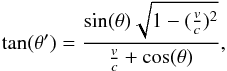
Two effects have to be taken into account. The emitted radio frequency
frest is observed at the Doppler shifted frequency
fobs. The magnitude of this change depends on the angle
θ between the direction to the source and the direction of our motion,
with velocity v. Observed and rest frame frequencies are related by
 (5)where δ
is given by
(5)where δ
is given by  (6)Thus the observed flux
changes due to our motion, since it depends on the frequency
(6)Thus the observed flux
changes due to our motion, since it depends on the frequency  (7)The first factor of
δ is due to the fact that the energy of an observed photon is enhanced
due to the Doppler effect.
(7)The first factor of
δ is due to the fact that the energy of an observed photon is enhanced
due to the Doppler effect.
Thus, the Doppler effect will change the number of observed sources above a given flux
limit like  (8)Since the velocity
of light is finite, aberration will also modify the number counts. The position of each
source is changed towards the direction of motion. The new angle
θ′ (observed from Earth) between the position of the source
and the direction of motion is given by
(8)Since the velocity
of light is finite, aberration will also modify the number counts. The position of each
source is changed towards the direction of motion. The new angle
θ′ (observed from Earth) between the position of the source
and the direction of motion is given by  (9)Therefore, at first order
in v/ c, dΩ
transforms like
(9)Therefore, at first order
in v/ c, dΩ
transforms like  (10)This can be combined with
the Doppler effect to give the observed number density. After approximating
δ(v,θ) to first order in
(10)This can be combined with
the Doppler effect to give the observed number density. After approximating
δ(v,θ) to first order in
 , the
result becomes
, the
result becomes ![\begin{equation} \label{numbercountapprox} \frac{{\rm d}N}{{\rm d}\Omega}_{\mathrm{obs}} = \left(\frac{{\rm d}N}{{\rm d}\Omega}\right)_{\mathrm{rest}} \left[1+[2+x(1+\alpha)] \left(\frac{v}{c}\right) \cos(\theta)\right] . \end{equation}](/articles/aa/full_html/2013/07/aa21215-13/aa21215-13-eq54.png) (11)The amplitude of
the kinetic radio dipole is then given by
(11)The amplitude of
the kinetic radio dipole is then given by ![\begin{equation} \label{amplitudedefinition} d = [2+x(1+\alpha) ] \left(\frac{v}{c}\right)\cdot \end{equation}](/articles/aa/full_html/2013/07/aa21215-13/aa21215-13-eq55.png) (12)The kinetic radio
dipole points towards the direction of our peculiar motion, which in an isotropic and
homogeneous Universe must also agree with the direction defined by the CMB dipole.
(12)The kinetic radio
dipole points towards the direction of our peculiar motion, which in an isotropic and
homogeneous Universe must also agree with the direction defined by the CMB dipole.
2.2. Expected kinetic radio dipole
The measured CMB dipole is ΔT = 3.355 ± 0.008 mK in the direction (l,b) = (263.99° ± 0.14°,48.26° ± 0.03°) (Hinshaw et al. 2009). In equatorial coordinates (epoch J2000) its direction reads (RA, Dec) = (168°,−7°). Compared to the CMB temperature of T0 = 2.725 ± 0.001 K (Fixsen & Mather 2002). this corresponds to a relative fluctuation of ΔT/ T = (1.231 ± 0.003) × 10-3 and thus the velocity of the Solar system has been inferred from the CMB dipole to be v = 369.0 ± 0.9 km s-1 (Hinshaw et al. 2009).
To find the expected amplitude of the kinetic radio dipole, we also need estimates for x and α. The typically assumed values are x = 1 and α = 0.75, which gives together with v = 370 km s-1 a radio dipole amplitude of d = 0.46 × 10⁻². However, we can improve on that as x can be measured with help of the radio survey. Therefore we need to plot N(> S) against S like in Fig. 1.
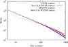 |
Fig. 1 Number counts of the NVSS and WENSS surveys. A function f(S) ∝ S− x is fitted to both data sets in the range of 25 mJy < S < 200 mJy. Resulting values of x are 1.10 ± 0.02 for the NVSS survey and 0.80 ± 0.02 for the WENSS survey. |
For the purpose of this work we find xNVSS = 1.10 ± 0.02 and xWENSS = 0.80 ± 0.02. The mean spectral index cannot be inferred from the catalogues, as they provide data at a single frequency band only. We thus stick to α = 0.75, but include in the dipole error an uncertainty of Δα = 0.25 (Garn et al. 2008). This results in the expectations:
![\begin{eqnarray} &&d_{\rm NVSS}^{\rm exp} = (0.48 \pm 0.04) \times 10^{-2}, \\[3mm] &&d_{\rm WENSS}^{\rm exp} = (0.42 \pm 0.03) \times 10^{-2}. \end{eqnarray}](/articles/aa/full_html/2013/07/aa21215-13/aa21215-13-eq78.png)
The error is dominated by the uncertainty in the spectral index.
3. Previous results
The first measurement of the radio dipole using the NVSS catalogue was performed by Blake & Wall (2002). In order to remove corruption
by local structure, all sources within 15° vicinity of the Galactic disk have
been removed. Additionally the clustering dipole contribution was reduced by ignoring
sources within 30′′ of nearby known galaxies. The spherical harmonic coefficients
 from the
remaining NVSS catalogue have been determined up to l = 3. A model for a
dipole distribution with an isotropic background has been constructed
(a00 and a10). Due to masking,
this dipole distribution also influences higher multipoles. After applying the same mask as
for the NVSS catalogue, one finds
from the
remaining NVSS catalogue have been determined up to l = 3. A model for a
dipole distribution with an isotropic background has been constructed
(a00 and a10). Due to masking,
this dipole distribution also influences higher multipoles. After applying the same mask as
for the NVSS catalogue, one finds  up to
l = 3. A quadratic estimator (chi square) was used to compare the model
with the observed coefficients.
up to
l = 3. A quadratic estimator (chi square) was used to compare the model
with the observed coefficients.
The resulting best-fit dipoles can be seen in Table 1. The results of Blake & Wall (2002) indicate a higher radio dipole than expected, however without statistical significance.
Best-fit dipole parameters from Blake & Wall (2002).
Singal (2011) used a linear estimator, originally
proposed by Crawford (2009),  (15)and a variation of it,
which we discuss below. For a large number of sources the isotropic background will clear
away. The remaining vector R3D will point towards
the main anisotropy in the distribution of number density over the sky. To get the correct
dipole amplitude d one has to normalize this estimator depending on the
number of sources. In Singal’s analysis sources within 10° of the Galactic plane
have been removed. In order to avoid directional bias (see the more detailed discussion
below), he reestablished a north-south symmetry of the NVSS by cutting all sources with
dec > 40°. The results of Singal (2011) are shown in Table 2. The errors of the directional measurements are quite small here. This is an
effect of an unexpectedly large amplitude, which simplifies the measurement. While the
direction agrees with the one found by Blake & Wall
(2002), the dipole amplitude seems to be a factor of about four higher than
expected from the CMB dipole and twice as big as found by Blake & Wall (2002).
(15)and a variation of it,
which we discuss below. For a large number of sources the isotropic background will clear
away. The remaining vector R3D will point towards
the main anisotropy in the distribution of number density over the sky. To get the correct
dipole amplitude d one has to normalize this estimator depending on the
number of sources. In Singal’s analysis sources within 10° of the Galactic plane
have been removed. In order to avoid directional bias (see the more detailed discussion
below), he reestablished a north-south symmetry of the NVSS by cutting all sources with
dec > 40°. The results of Singal (2011) are shown in Table 2. The errors of the directional measurements are quite small here. This is an
effect of an unexpectedly large amplitude, which simplifies the measurement. While the
direction agrees with the one found by Blake & Wall
(2002), the dipole amplitude seems to be a factor of about four higher than
expected from the CMB dipole and twice as big as found by Blake & Wall (2002).
Masking the supergalactic plane in order to reduce the contribution of local structure did not resolve the discrepancy. Since unknown clustering further away from the super Galactic plane could also have contributed to the measurement, a second test was performed. A clustering contribution to the dipole would not give a signal proportional to cosθ. On the other hand, the difference in number counts of areas that are opposite to each other should decrease with cosθ (where θ is the angle between an area and the measured dipole direction), if the measured dipole is due to our velocity. Singal was able to fit such a behaviour to the data. Therefore he concludes that the radio dipole amplitude is not due to local clustering.
Dipole direction and amplitude from the number count estimator (15) from Singal (2011).
Singal (2011) also used a linear estimator for the
distribution of flux over the sky. This estimator is similar to the number density estimator
(15), but weights each radio source by its
flux Si,  (16)Like
R3D, this estimator finds the main anisotropy
and the amplitude needs to be normalized. The brightest sources
(S > 1000 mJy) are removed, because they would
dominate Rflux otherwise. Results of this estimator
are shown in Table 3. The estimated directions are in
agreement with the results of Blake & Wall
(2002) and the number count estimator results of Singal (2011). However, the normalized dipole amplitudes d are
even higher than those of the number count estimator
R3D. In Sect. 6 we resolve this conflict.
(16)Like
R3D, this estimator finds the main anisotropy
and the amplitude needs to be normalized. The brightest sources
(S > 1000 mJy) are removed, because they would
dominate Rflux otherwise. Results of this estimator
are shown in Table 3. The estimated directions are in
agreement with the results of Blake & Wall
(2002) and the number count estimator results of Singal (2011). However, the normalized dipole amplitudes d are
even higher than those of the number count estimator
R3D. In Sect. 6 we resolve this conflict.
Dipole direction and amplitude from the flux weighted number count estimator (16) from Singal (2011).
Most recently, Gibelyou & Huterer (2012)
measured a dipole amplitude (d = 2.7 ± 0.5) × 10-2 towards (RA,
Dec) = (117 ± 20°,6 ± 14°) from the NVSS. This
direction is inconsistent with the studies mentioned above and the dipole amplitude is a
factor of five larger than expected. The authors used separate estimators for the direction
and the amplitude. Their direction estimate is based on a linear estimator, originally
proposed by Hirata (2009),  (17)This
three-dimensional estimator (3DM) is intended to be unbiased for arbitrary survey geometries
and arbitrary masking. The idea is to achieve that with help of the second sum, which goes
over NR randomly distributed points, subject to the same
masking. Therefore, the authors include all sources of the NVSS survey, except for those
within 10° of the Galactic plane. Below we show that this estimator has a
direction bias, which depends on the real dipole anisotropy.
(17)This
three-dimensional estimator (3DM) is intended to be unbiased for arbitrary survey geometries
and arbitrary masking. The idea is to achieve that with help of the second sum, which goes
over NR randomly distributed points, subject to the same
masking. Therefore, the authors include all sources of the NVSS survey, except for those
within 10° of the Galactic plane. Below we show that this estimator has a
direction bias, which depends on the real dipole anisotropy.
We summarize, there is no agreement on the amplitude and direction of the cosmic radio dipole so far.
4. Linear estimators for a full sky
Let us first show that the estimator (15) provides an unbiased estimate of the dipole direction.
Starting from the distribution of the number of radio sources per solid angle (11), as seen by a moving observer in an
otherwise isotropic Universe, the probability to find a given radio source within a solid
angle dΩ of position  is given by
  (18)where
d denotes the dipole vector.
(18)where
d denotes the dipole vector.
To study the bias of an estimator, we calculate its expectation value with respect to an
ensemble average. We do so below by means of Monte Carlo studies. For analytic
considerations, for large N we replace the ensemble average by a spatial
average, i.e.  (19)thus we assume
ergodicity. Note that the average is a linear operator.
(19)thus we assume
ergodicity. Note that the average is a linear operator.
Now the expectation value of Crawford’s estimator can be evaluated for large
N,  (20)This calculation holds for
independent, identically distributed positions
(20)This calculation holds for
independent, identically distributed positions  ,
thus without clustering effects. Only the second term survives the integration and thus the
expected dipole estimator is
,
thus without clustering effects. Only the second term survives the integration and thus the
expected dipole estimator is  (21)Naively, one could now
estimate the dipole signal by
(21)Naively, one could now
estimate the dipole signal by  .
.
We conclude that d3D provides us with an unbiased
estimate of the dipole direction  for a full sky sample. However the estimated dipole amplitude
| d3D | is biased.
for a full sky sample. However the estimated dipole amplitude
| d3D | is biased.
To understand the origin of this bias let us first consider  (22)The inequality holds for
large N and d < 3 (in case of
large dipole amplitudes [
(22)The inequality holds for
large N and d < 3 (in case of
large dipole amplitudes [ ]
our ansatz (19) should also take many-point
correlations into account). Thus
]
our ansatz (19) should also take many-point
correlations into account). Thus  is definitely
biased towards higher amplitudes. However, to prove that
| d3D | is biased, we would need to calculate
⟨| d3D |⟩. We do this by means of the random
walk/flight method.
is definitely
biased towards higher amplitudes. However, to prove that
| d3D | is biased, we would need to calculate
⟨| d3D |⟩. We do this by means of the random
walk/flight method.
4.1. Random flight
Adding up vectors for each point of a survey corresponds to a random walk with unit step size. To be more precise this is a random flight, since the problem is three dimensional. Even for a vanishing dipole, such a random flight is unlikely to return to the origin after N steps. This describes the noise of any realisation of an isotropic distribution of N sources.
Following Crawford (2009), we determine the
distance r from the origin after N steps from the
probability density of a random flight process ![\begin{equation} \label{Result3DFlight} \check{P}_N(r) \mathrm{d}r= \left[ \frac{54}{\pi N^3}\right]^{1/2} r^2 \exp\left( -\frac{3 r^2}{2N} \right) \mathrm{d}r. \end{equation}](/articles/aa/full_html/2013/07/aa21215-13/aa21215-13-eq193.png) (23)The probability of
measuring a dipole signal of an amplitude bigger than R in a random
flight is
(23)The probability of
measuring a dipole signal of an amplitude bigger than R in a random
flight is  (24)A confidence level
pCL can be choosen, leading to errorbars for a measured dipole vector
R3D ± RpCL. To
estimate the directional uncertainties of this method, Crawford (2009) made the following argument: at a given confidence level the
random flight corresponds to a step of length up to
RpCL. Adding
RpCL perpendicular to the measured dipole
R3D allows us to estimate the maximal offset
in direction. Using trigonometry, one can relate
RpCL to the directional uncertainties
expressed as the angle
(24)A confidence level
pCL can be choosen, leading to errorbars for a measured dipole vector
R3D ± RpCL. To
estimate the directional uncertainties of this method, Crawford (2009) made the following argument: at a given confidence level the
random flight corresponds to a step of length up to
RpCL. Adding
RpCL perpendicular to the measured dipole
R3D allows us to estimate the maximal offset
in direction. Using trigonometry, one can relate
RpCL to the directional uncertainties
expressed as the angle  (25)The expected magnitude of
the random dipole contribution is estimated from (23) as
(25)The expected magnitude of
the random dipole contribution is estimated from (23) as ![\begin{equation} \label{estimateA} \langle R_{\mathrm{3D}}^{\mathrm{random}} \rangle= \int_0^\infty r \left[ \frac{54}{\pi N^3}\right]^{1/2} r^2 \exp\left( -\frac{3 r^2}{2N} \right) \mathrm{d}r \approx 0.92 \sqrt{N} . \end{equation}](/articles/aa/full_html/2013/07/aa21215-13/aa21215-13-eq201.png) (26)Since the random dipole
has no distinguished direction, there is no direction bias of the linear estimator for a
full sky map.
(26)Since the random dipole
has no distinguished direction, there is no direction bias of the linear estimator for a
full sky map.
 |
Fig. 2 Ampliude bias of the full sky estimator d3D. Data
represent mean and empirical variance of 1000 simulations for each
N. A function |
Even for vanishing d, this gives rise to a non-vanishing estimate of the
dipole amplitude  and is
thus the origin of the amplitude bias.
and is
thus the origin of the amplitude bias.
Motivated by (22) we make the following
ansatz for the dipole amplitude and its bias:  (27)To verify this analytic
estimate of the biased amplitude, we simulated full sky maps including a velocity dipole
(with v = 370 km s-1). From these simulated catalogues we
extracted the observed amplitude dobs. Figure 2 shows the simulated data, the true value of the dipole
amplitude and a fit of the form
(27)To verify this analytic
estimate of the biased amplitude, we simulated full sky maps including a velocity dipole
(with v = 370 km s-1). From these simulated catalogues we
extracted the observed amplitude dobs. Figure 2 shows the simulated data, the true value of the dipole
amplitude and a fit of the form  .
.
The best-fit values are A = 0.908 ± 0.002 and D = (0.451 ± 0.001) × 10-2 (statistical errors only). These numbers should be compared to the factor 0.92 from (26) and the simulation input of d = 0.46 × 10⁻². The reduced chi- square of the fit is 7 × 10⁻⁵. Thus the Monte Carlo simulations agree with the theoretically motivated ansatz (27) for the expected dipole amplitude of the estimator d3D.
We conclude that even for a perfect full sky catalogue (no masking, complete in flux, perfect flux and position measurements), the amplitude of the linear estimator is biased towards higher values. Increasing the number of radio sources will reduce the bias. The estimator d3D is asymptotically unbiased, but this is of limited practical use for the analysis of NVSS and WENSS data. A similar bias of the dipole amplitude is also found for the other linear estimators introduced above. This finding is in agreement with Gibelyou & Huterer (2012), who use a linear estimator to find the direction of the dipole.
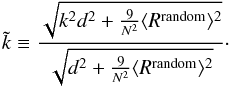
5. Linear estimators for an incomplete sky
So far we assumed full coverage of the radio sky. More realistic catalogues cover just a fraction of the sky, as all earth based telescopes are limited to observe at certain declination ranges. Additionally, the Milky Way is masking parts of the sky. Here we discuss some of the effects caused by incomplete sky coverage.
The upcoming Low Frequency Array (LOFAR) Tier-1 survey will cover about half of the sky (2π), thus we first focus on this situation. As a second step we generalize this to an arbitrary axisymmetric survey geometry and include the effects of masking.
5.1. Random walk
Let us assume a survey geometry that covers all of the Northern hemisphere and ask how
the estimator of the radio dipole (15) has
to be modified. For the first two Cartesian components of
R3D there should be no systematic problem, but
the third component will definitely be biased. It is necessary to remove the effect of the
incomplete sky from this z component. Consider the expectation value of
R3D for the Northern hemisphere
 (28)where
pd ≡ 1/ [1 + (d/ 2)cosϑd)]
accounts for the proper normalisation of the probability distribution on the hemisphere in
presence of a dipole. 4π in (18) becomes 2π for obvious reasons. The integral can be
evaluated by hand. One finds
(28)where
pd ≡ 1/ [1 + (d/ 2)cosϑd)]
accounts for the proper normalisation of the probability distribution on the hemisphere in
presence of a dipole. 4π in (18) becomes 2π for obvious reasons. The integral can be
evaluated by hand. One finds  (29)where
ϑd and ϕd denote the dipole
position in spherical coordinates. The z direction is strongly influenced
by the incomplete sky coverage. The total number of observed sources is not independent
from the amplitude and orientation of the dipole itself.
(29)where
ϑd and ϕd denote the dipole
position in spherical coordinates. The z direction is strongly influenced
by the incomplete sky coverage. The total number of observed sources is not independent
from the amplitude and orientation of the dipole itself.
Nevertheless there is no problem in the evaluation of ϕd
because one can calculate  (30)Here
N as well as sinϑd cancel out. So the 2D
estimator is unbiased with respect to ϕd. Therefore we propose
a pure two dimensional estimator:
(30)Here
N as well as sinϑd cancel out. So the 2D
estimator is unbiased with respect to ϕd. Therefore we propose
a pure two dimensional estimator:  (31)From this one can still
use
(31)From this one can still
use  for
evaluating
dsinϑdNpd/ 3
and ϕd. Let us take a look at the factor
sinϑd. Sources near the pole will make a smaller
contribution than those further away. If a source near the pole is shifted by a small
distance, the value ϕi of this source could
change dramatically. So the weighting terms compensate for this artificially big errors,
which are just a relic of the coordinate system.
for
evaluating
dsinϑdNpd/ 3
and ϕd. Let us take a look at the factor
sinϑd. Sources near the pole will make a smaller
contribution than those further away. If a source near the pole is shifted by a small
distance, the value ϕi of this source could
change dramatically. So the weighting terms compensate for this artificially big errors,
which are just a relic of the coordinate system.
Let us now estimate the uncertainties of the estimator
R2D. The problem corresponds to an isotropic
random walk process with variable step size. The probability density for a displacement of
r for such a random walk is  (32)Similar to the random
flight we determine RpCL defined by
(32)Similar to the random
flight we determine RpCL defined by
 (33)Here again
pCL is the confidence level. It is possible to solve the above integral
analytically
(33)Here again
pCL is the confidence level. It is possible to solve the above integral
analytically 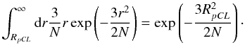 (34)So
RpCL is given by
(34)So
RpCL is given by 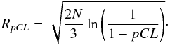 (35)Now one can use the same
argument as for the random flight to evaluate the uncertainty of the
ϕd estimation
(35)Now one can use the same
argument as for the random flight to evaluate the uncertainty of the
ϕd estimation  (36)In this way one can
directly determine error bars for measured results of ϕd
calculated via (30). Using this two
dimensional estimator one cannot measure the dipole amplitude d itself
but only the combination
dsinϑdNpd/ 3.
Therefore it can only give an lower limit for d.
(36)In this way one can
directly determine error bars for measured results of ϕd
calculated via (30). Using this two
dimensional estimator one cannot measure the dipole amplitude d itself
but only the combination
dsinϑdNpd/ 3.
Therefore it can only give an lower limit for d.
Like in the case of the full three dimensional estimator, this version is also biased in
the measurement of the amplitude. The expectation of the random contribution can be
calculated via 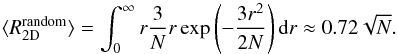 (37)So we expect our
estimator to measure a combination of this random contribution and the true velocity
dipole and make the ansatz
(37)So we expect our
estimator to measure a combination of this random contribution and the true velocity
dipole and make the ansatz  (38)where we used
pd ≈ 1. Like above, we verify this via Monte Carlo
simulations, shown in Fig. 3.
(38)where we used
pd ≈ 1. Like above, we verify this via Monte Carlo
simulations, shown in Fig. 3.
 |
Fig. 3 Ampliude bias for the estimator d2D on a hemisphere.
Data represent mean and empirical variance of 1000 simulations for each N. A
function |
5.2. Direction bias
For any masked or incomplete map of the sky, we cannot measure the mean source density
 ,
i.e. the monopole. Therefore we always have to keep in mind that the observed mean density
is just an approximation. Gibelyou & Huterer
(2012) have used an estimator proposed by Hirata
(2009), which implicitly assumes, that the monopole is known. Based on the
knowledge of the monopole, this estimator would compensate for masking effects and
incomplete sky coverage by substracting a pure random isotropic map from the observed
dipole term via (17). However, we cannot
know
,
i.e. the monopole. Therefore we always have to keep in mind that the observed mean density
is just an approximation. Gibelyou & Huterer
(2012) have used an estimator proposed by Hirata
(2009), which implicitly assumes, that the monopole is known. Based on the
knowledge of the monopole, this estimator would compensate for masking effects and
incomplete sky coverage by substracting a pure random isotropic map from the observed
dipole term via (17). However, we cannot
know  .
.
For the previous example of a hemisphere, the monopole density is
 ,
where N = ND in (17). The random map can be made up of an
arbitrary number of sources NR, but is reweighted by the
observed number of sources
ND/ NR,
instead of
,
where N = ND in (17). The random map can be made up of an
arbitrary number of sources NR, but is reweighted by the
observed number of sources
ND/ NR,
instead of  .
This introduces a directional bias, in addition to the previously discussed biased
amplitude. One can see this explicitly by applying (17) on our model of a dipole modified isotropic hemisphere. We find
.
This introduces a directional bias, in addition to the previously discussed biased
amplitude. One can see this explicitly by applying (17) on our model of a dipole modified isotropic hemisphere. We find
 (39)which clearly is not
parallel to d. For small values of d we can
expand pd and obtain
(39)which clearly is not
parallel to d. For small values of d we can
expand pd and obtain
 (40)The
z component of the dipole is underestimated by a factor of 4 for the
geometry of a hemisphere. Despite cancelation of the leading term of the bias of the
z direction, the dipole direction remains biased. Less symmetric survey
geometries lead to a bias of all dipole components for this estimator.
(40)The
z component of the dipole is underestimated by a factor of 4 for the
geometry of a hemisphere. Despite cancelation of the leading term of the bias of the
z direction, the dipole direction remains biased. Less symmetric survey
geometries lead to a bias of all dipole components for this estimator.
The best strategy to avoid any directional bias for a linear estimator is to make the survey geometry point symmetric around the observer for three dimensional estimators like R3D or point symmetric around the zenith in case of two dimensional estimators R2D. This implies for the NVSS that one has to cut symmetric in declination, such that both polar caps are missing, a strategy that was used by Singal (2011).
5.3. Masking
The use of a masked sky additionally affects the dipole measurement. In general, the estimated dipole direction and amplitude depend on the position of the true dipole relative to the mask. Cutting areas with large dipole contribution will reduce the amplitude and vice versa.
In the following we consider masks that are point symmetric with respect to the observer for all considered 3-dimensional estimators, respectively point symmetric with respect to the zenith for the 2-dimensional estimators. Constructed in such a way, masking does not introduce any directional bias. Nevertheless, we have to consider the effects of masking on the estimated dipole amplitude.
A simple method to correct for this effect was put forward by Singal (2011), who introduced a masking factor k,
 (41)Such a factor is
expected to be a function of shape and position of the mask as well as the dipole
position. In most cases an analytic calculation of this factor is impossible. For simple
mask geometries some analytic results can be found in Rubart (2012). An alternative approach is to simulate the effects by means of
Monte Carlos and to compare simulations with and without masking. The ratio of both
results after a large number of simulations provides the masking factor
k3D.
(41)Such a factor is
expected to be a function of shape and position of the mask as well as the dipole
position. In most cases an analytic calculation of this factor is impossible. For simple
mask geometries some analytic results can be found in Rubart (2012). An alternative approach is to simulate the effects by means of
Monte Carlos and to compare simulations with and without masking. The ratio of both
results after a large number of simulations provides the masking factor
k3D.
Doing so, we found some interesting effects. The masking factors depend on the number of
objects in the simulated maps as well as on the true dipole amplitude. This can be
explained as follows. The masking will mainly affect the kinetic dipole contribution,
while the random dipole will increase due to the decrease of the number of objects in the
masked catalogue. Therefore we expect the amplitude to be  (42)k3D
should only depend on the properties of the mask and not on the amplitude of the dipole.
To test this, we created simulated maps for two different dipole amplitudes, with values
motivated by the CMB measurement dCMB = 0.46 × 10⁻²
and by the measurement of Blake & Wall
(2002) at 25 mJy dBW = 1.1 × 10⁻². We used
the direction RA = 158°,Dec = −4° in both cases.
The mask agrees with the one used by Singal (2011),
i.e. we removed all sources with
| δ| > 40° and
| b| < 10°. Resulting amplitudes
for different numbers of sources are shown in Fig. 4.
(42)k3D
should only depend on the properties of the mask and not on the amplitude of the dipole.
To test this, we created simulated maps for two different dipole amplitudes, with values
motivated by the CMB measurement dCMB = 0.46 × 10⁻²
and by the measurement of Blake & Wall
(2002) at 25 mJy dBW = 1.1 × 10⁻². We used
the direction RA = 158°,Dec = −4° in both cases.
The mask agrees with the one used by Singal (2011),
i.e. we removed all sources with
| δ| > 40° and
| b| < 10°. Resulting amplitudes
for different numbers of sources are shown in Fig. 4.
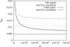 |
Fig. 4 Amplitude bias of the 3-dimensional estimator for the masked NVSS geometry of Singal (2011). Data represent mean and empirical
variance of 1000 simulations for each N. A function
|
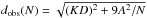
First of all we can conclude that (42) is a good fit for the behaviour of the simulated maps in both cases. The measured amplitudes are larger than those estimated from full sky maps. We can now calculate k3D. In both cases it turns out to be 1.4, which could be used to correct the amplitude estimate.
A similar argument holds for the two dimensional estimator. Here we expect a behaviour of
the form:  (43)Using the same
assumptions about the dipole term and the same mask as before, we obtain Fig. 5.
(43)Using the same
assumptions about the dipole term and the same mask as before, we obtain Fig. 5.
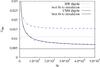 |
Fig. 5 Amplitude bias of the 2-dimensional estimator for the masked NVSS geometry of Singal (2011). Data represent mean and empirical
variance of 1000 simulations for each N. A function
|
This time, we find k2D = 1.3 for both assumed velocities. The simulations support our assumption that the masking factor does not depend on the dipole magnitude d.
5.3.1. Masking correction
Although the masking factor k does not depend on the amplitude
d, it may depend on the dipole direction
 .
Therefore it would be necessary to repeat the analysis of the previous section for each
dipole direction found. To reduce the simulation effort, we rely on the following method
instead.
.
Therefore it would be necessary to repeat the analysis of the previous section for each
dipole direction found. To reduce the simulation effort, we rely on the following method
instead.
For the full, as well as for the masked sky, surveys with 106 sources were
simulated. This choice guarantees that we investigate masking effects and not effects
due to shot noise. The mean dipole amplitudes are determined for 103
simulated full and masked sky surveys, respectively. The ratio of the masked sky mean
amplitude to the full sky mean amplitude is denoted
 .
This ratio provides a first approximation to the masking factor.
.
This ratio provides a first approximation to the masking factor.
 (44)The influence of the
random dipole tends to bias
(44)The influence of the
random dipole tends to bias  towards 1 (as can be easily seen in the limit of a small number of sources). This bias
can be compensated by rewriting the above formula into
towards 1 (as can be easily seen in the limit of a small number of sources). This bias
can be compensated by rewriting the above formula into
 (45)The values of
N and d are input parameters of the simulation. From
the last section we know the values of ⟨ Rrandom ⟩ for the
three- as well as for the two-dimensional case. Therefore we can transform the
approximated masking factor
(45)The values of
N and d are input parameters of the simulation. From
the last section we know the values of ⟨ Rrandom ⟩ for the
three- as well as for the two-dimensional case. Therefore we can transform the
approximated masking factor  into the unbiased masking factor k.
6. Dipole from a flux weighted estimator
Let us now turn to a discussion of the flux weighted estimator (16), which was used by Singal (2011).
We first take a closer look at the theoretically expected value of the flux dipole
dflux. For simplicity we assume full sky
coverage. For a large number of sources,
 (46)where
θ is the angle between a source and the dipole direction
(46)where
θ is the angle between a source and the dipole direction
 .
.
We now determine the number of sources per flux and solid angle as a function of the
observer velocity. At zeroth order in velocity, this density
n(S) is isotropic. As for the number counts, stellar
aberration and the Doppler effect have to be taken into account. Stellar aberration gives
rise to  (47)The relativistic
Doppler effect alters the observed fluxes. When we observe a source in the direction of
motion, we measure a higher flux than if we were at rest with respect to the isotropic and
homogeneous Universe. We relate the observed flux S0 to the flux
that is measured by an observer with vanishing peculiar motion,
(47)The relativistic
Doppler effect alters the observed fluxes. When we observe a source in the direction of
motion, we measure a higher flux than if we were at rest with respect to the isotropic and
homogeneous Universe. We relate the observed flux S0 to the flux
that is measured by an observer with vanishing peculiar motion,
 (48)We assume the power law
 to hold for observers at rest and Taylor expand around the observed flux
![\begin{equation} n(S_{\rm rest}) \approx n(S_0)\left[1 + \tilde x (1+\alpha)\frac{v}{c} \cos \theta \right] . \end{equation}](/articles/aa/full_html/2013/07/aa21215-13/aa21215-13-eq297.png) (49)If the assumed power
law holds for all sources of a survey, then
(49)If the assumed power
law holds for all sources of a survey, then  , with x as
defined above in (4). Combining the Doppler
effect and the stellar aberration leads to
, with x as
defined above in (4). Combining the Doppler
effect and the stellar aberration leads to
![\begin{equation} \frac{\mathrm{d}^2N}{\mathrm{d} \Omega \mathrm{d}S} =n_0(S_0)\left[1+(2+\tilde x (1+\alpha))\frac{v}{c}\cos \theta\right] + O \left( \left( \frac{v}{c}\right)^2 \right) \cdot \end{equation}](/articles/aa/full_html/2013/07/aa21215-13/aa21215-13-eq299.png) (50)This result only holds
under the assumption of a power law behaviour of the number counts. It is crucial to keep
this in mind.
(50)This result only holds
under the assumption of a power law behaviour of the number counts. It is crucial to keep
this in mind.
6.1. NVSS
Let us now see, if we are allowed to make this assumption for the analysis of NVSS data. The plot in Fig. 6 demonstrates that the power law is not valid for the flux range used in the analysis of Singal (2011), i.e. fluxes up to 1 Jy. Actually the slope steepens for the larger fluxes considered. The best fit power-law gives a reduced chi-squared value of χ2 = 122. That means that the observed data cannot be fitted by a power law.
Thus Singal’s assumption  does not hold for two reasons.
Firstly, for a pure power law we would expect
does not hold for two reasons.
Firstly, for a pure power law we would expect  , which is close to what we
find:
, which is close to what we
find:  . Secondly, the power-law
assumption only applies to about one half of the data.
. Secondly, the power-law
assumption only applies to about one half of the data.
 |
Fig. 6 Differential number counts of the NVSS catalogue,
Smin = 10 mJy, best fit values for
|

In conclusion, the result of unexpectedly large amplitudes in Singal (2011) could partly be explained by this two effects. With power
law behaviour one should use  or larger to also account
for the steepening of the spectral index at high fluxes, which increases the expectation
value by
or larger to also account
for the steepening of the spectral index at high fluxes, which increases the expectation
value by 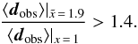 (51)The results of
the flux weighted estimator from Singal (2011)
should be reduced by at least a factor of 1.4.
(51)The results of
the flux weighted estimator from Singal (2011)
should be reduced by at least a factor of 1.4.
Compared to the estimator of Crawford, the estimator (16) stresses sources with high flux. To avoid the domination of a small number of sources, sources with S > 1000 mJy are not taken into account. Nevertheless, this estimator is stressing bright sources. These sources are, on average, nearer than the rest. Hence (16) might be dominated by nearby sources and by atypically bright ones. This seems to be yet another weakness of this estimator, since the local universe is anisotropic.
7. Dipole estimates from NVSS and WENSS
7.1. 3D linear estimates
We are now in a position to check the three dimensional estimations of the radio dipole in the NVSS catalogue. As we have shown above, the estimator used by Gibelyou & Huterer (2012) (17) gives rise to a biased dipole direction and thus is not further considered in this work. The flux weighted estimator (16) is also of limited use, as the NVSS data cannot be described by a power-law over all fluxes of interest. We thus focus here on the simplest linear estimator (15).
In order to obtain an unbiased direction estimate, the cut sky geometry of Singal (2011) is adopted. The masking factor
k is determined for every measured dipole anisotropy direction, as
described in 5.3.1. The pure estimator results
d3D are then corrected for the masking bias and we obtain
 .
.
Dipole direction and amplitude from NVSS.
All results for right ascension agree within their error bars. The same holds true for the dipole amplitudes. This self-consistency indicates the absence of significant systematic errors. Unfortunately, we can not state the same for the declination results. One observes an significant increase in declination with respect to deceasing flux limits. This effect is very likely due to a relic of the NVSS survey procedure. Sources below δ = −10° were measured by means of a different alignment of the Very Large Array. The source density is therefore smaller in this area. Therefore it is expected that the dipole measurement will show increasing values of declination at the fainter flux limits. This makes it hard to trust the declination results below a flux limit of 25 mJy (note that there is no significant difference between 20 mJy and 30 mJy).
The results of Table 4 can be compared to those in Table 2. Number of sources and direction results are almost the same. Deviations could be explained by minor differences in the precise form of the mask. We used a different method for estimating uncertainties in the direction and amplitude measurement, than those used by Singal (2011). Since our method (described above) is more conservative, we obtain larger errorbars. All dipole amplitudes in this table are slightly below those from Table 2. In Singal (2011) a different method was used to obtain the dipole amplitude from the estimator (15), which can explain this discrepancy. In principle we can recover the results of Singal (2011) and confirm an unexpectedly high dipole amplitude.
7.2. 2D linear estimates
A disadvantage of the NVSS catalogue is that the sampling depth changes at δ = −10° (less sensitivity at lower declinations). This could lead to a directional bias of the NVSS data analysis and thus it is interesting to also use the two dimensional estimator presented in this work, as this effect cannot lead to a bias in this case. For the WENSS analysis, a three dimensional linear estimator cannot avoid directional bias.
7.2.1. NVSS
A major advantage of the estimator R2D is that it does not require a north-south symmetry of the catalogue. Therefore, the declination limit of the NVSS catalogue is no problem.
As the estimator R2D requires a point symmetry around the north pole, we cannot remove the Galactic plane only. For each removed point we also need to subtract the point which is 180° away. When we do so, a second plane occurs, which we call the counter Galactic plane (CG). A HEALPix1 map of the remaining NVSS sources can be seen in Fig. 7. The colour of the pixels encodes the number of sources per pixel.
 |
Fig. 7 Map of the number counts in HEALPix pixels from NVSS. The pixel size corresponds to Nside = 32. Shown are equatorial coordinates at epoch J2000. The NVSS contains data at δ > −40° and the Galactic plane and a “counter galaxy” are masked (CG mask) in order to avoid Galactic contamination and to restore point symmetry with respect to the zenith. |
An alternative would be the mask used by Singal (2011). That mask is a combination of two great cycles and would therefore also work for R2D. However, it turns out that the mask with the CG removes fewer sources. Thus we decided to use the CG mask.
The next step is to evaluate the masking correction k of the CG mask. As this factor depends on the right ascension and on the declination of the dipole anisotropy, we need some additional information. From R2D we estimate the right ascension. As the declination cannot be evaluated with R2D, we use the declination as provided by the three dimensional estimator in order to determine k. These values are certainly not exact, since a different mask is used now. The influence of a small change in dipole declination on the evaluated factor k is discussed in Sect. 7.2.2.
We reduce the dipole amplitude of the 2D estimator by the masking factor
k and obtain the masking corrected amplitude
 . The
results of this procedure for the NVSS catalogue and different flux limits can be found
in Table 5.
. The
results of this procedure for the NVSS catalogue and different flux limits can be found
in Table 5.
Dipole right ascension and amplitude dsinθd from NVSS.
Obtained right ascensions and amplitudes are stable with respect to different flux limits. For all flux limits ≥15 mJy, the estimated right ascension of the radio dipole is in agreement with the CMB prediction of RA = 168°. Only when we include sources as faint as 10 mJy, we find a 3σ deviation. However, we know that the catalogue is incomplete at its faint end.
The masking corrected dipole amplitudes  are
significantly above the CMB prediction. To some extent this is expected due to the
discussed amplitude bias. A detailed discussion is presented in the next section.
are
significantly above the CMB prediction. To some extent this is expected due to the
discussed amplitude bias. A detailed discussion is presented in the next section.
7.2.2. WENSS
We finally present the first estimation of the radio dipole from the WENSS catalogue. We cannot use the three dimensional linear estimators on this catalogue, since it only contains sources with Dec > 28°. The two dimensional estimator on the other hand can be used here. Again, we need to remove the Galactic plane and the counter Galactic plane to reestablish a symmetry around the north pole. The remaining WENSS catalogue is shown in Fig. 8.
 |
Fig. 8 Map of the number counts in HEALPix pixels from WENSS. The pixel size corresponds to Nside = 32. Shown are equatorial coordinates at epoch B1950. The WENSS contains data at δ > 30° and the Galactic plane and a “counter galaxy” are masked (CG mask) in order to avoid Galactic contamination and to restore point symmetry with respect to the zenith. |
To choose the best flux limit, we analyse the differential number counts between 10 mJy and 1000 mJy. Figure 9 shows that the WENSS catalogue seems to be incomplete below 25 mJy. In Rengelink et al. (1997) the completeness of the WENSS catalogue is claimed to hold only above a limit of 30 mJy. From Fig. 9 we infer that a simple power law also applies to the source counts between 25 and 30 mJy and thus we include sources down to a flux limit of 25 mJy in our analysis.
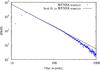 |
Fig. 9 Differential number counts of the WENSS catalogue,
Smin = 5 mJy, best fit values for
|

We cannot obtain information on the declination of the dipole from the WENSS catalogue by means of the two dimensional estimator applied in this work. This could in principle be a problem for the determination of the masking factor k. Therefore, we further investigated the effect of different dipole declinations. Assuming the WENSS symmetry and a right ascension of 120° (close to the results given in Table 7), we calculated k for 7 different values of declination, see Table 6. For this mask, the dependence of k on the right ascension of the dipole is relatively small, compared to shot noise uncertainties. We assume dec = 0° for the determination of k, based on the expectation from the CMB dipole and the NVSS radio dipole estimates.
Masking correction k for WENSS with CG mask and a dipole with RA = 120°.
Dipole estimate from WENSS based on 2D estimator using peak flux values for all sources with δ > 30°, except those in the Galactic and counter Galactic planes (CG mask).
The results of the WENSS analysis are presented in Table 7. Although the WENSS catalogue covers only one fourth of the sky, we find that it can be used for the estimation of the radio dipole. A problem is the limited number of sources that are left after masking the galaxy and restoring the required symmetry of the catalogue. This leads to larger error bars, compared with the NVSS estimates. We can conclude that the observed dipole anisotropy in the WENSS catalogue is in agreement with the measurements from NVSS, which is a nontrivial statement, as we are probing radio sources at different frequencies (325 MHz vs. 1.4 GHz).
8. Comparison of results
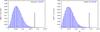 |
Fig. 10 Histogram of dipole amplitudes for 100,000 simulations of the three dimensional (left) and two dimensional (right) estimator, assuming the CMB expectation and a slope of x = 1.1, with 185 649 (left) and 195 245 (right) sources per simulation and appropriate masks. The black vertical lines are the NVSS results of this work. |
We summarize the various results from the literature and this work in Table 8. The results of this work are highlighted with bold faced letters. For comparison we focus on the flux limits of 25 mJy and 15 mJy.
All estimated dipole directions, both from the NVSS and from WENSS are in good agreement with each other and with the direction from the CMB dipole, with the exception of the result from Gibelyou & Huterer (2012). As explained in Sect. 5.2, their estimator shows a directional bias. We did not investigate any further, whether this bias invalidates their findings at a rather low flux limit. Our analysis based on the three dimensional estimator applied to NVSS and using the mask defined by Singal (2011) gives (RA, Dec) = (158° ± 19°,−2° ± 19°).
Comparison of results.
For the amplitude of the radio dipole, the situation is more contrived. Here we focussed on
the study of linear estimators and showed that all linear estimators under investigation
returned a biased estimate of the amplitude. The amplitude estimators of Blake & Wall (2002) and Gibelyou & Huterer (2012) are unbiased, but the latter one uses a
biased direction estimate as an input and is thus of limited interest. Besides bias, we
identified another effect that reduces the dipole amplitude found by the flux estimator used
in Singal (2011). We reduced the result of this
estimator by a factor of 1.4, due to the fact that the appropriate exponent of the
differential number count is given by  (see Sect. 6). With this correction, the result of the flux weighted estimator
(denoted by SIF* in Table 8) is now in agreement with
the result of Blake & Wall (2002).
(see Sect. 6). With this correction, the result of the flux weighted estimator
(denoted by SIF* in Table 8) is now in agreement with
the result of Blake & Wall (2002).
Our three dimensional estimate with the masking of Singal (2011) gives rise to d = (1.8 ± 0.6) × 10-2. One should keep in mind that this is a biased result, thus one cannot naively compare it to the expected amplitude. To figure out if our result is consistent with the null hypothesis that the radio sky is statistically isotropic, modified by the kinetic effects of our proper motion (measured via the CMB dipole), we performed 100 000 Monte Carlo simulations. The corresponding histogram is shown in Fig. 10. We find that only 21 of those realizations contain a dipole higher than the measured one and thus we can exclude that the estimated radio dipole is just due to our proper motion and amplitude bias at 99.6% CL. This is actually very puzzling, as the direction of the radio dipole agrees with the direction of the CMB dipole within the measurement error.
We can redo this analysis with the null hypothesis that the radio dipole was accurately measured by Blake & Wall (2002). This time we find that 3402 out of 100 000 realisations are higher than our measured dipole. If we increase the implemented velocity towards the upper one sigma bound of the dipole amplitude from Blake & Wall (2002), we observe every sixth simulation to be above our own measurement (16%). Therefore our result is in agreement with Blake & Wall (2002).
Before we turn to the discussion of potential explanations, let us inspect the dipole amplitudes from the two dimensional estimator. The dipole amplitudes estimated with the two dimensional estimator are also in agreement with the results of Singal (2011) and Blake & Wall (2002). We find dsinϑd = (1.9 ± 0.5) × 10-2 for the NVSS analysis and dsinϑd = (2.9 ± 1.9) × 10-2 for WENSS, which translate into lower limits on d. Thus, the results from the WENSS catalogue are in agreement with the radio dipole found in the NVSS catalogue. This is encouraging as they are prepared at different instruments and probe different frequencies.
In Figs. 10 and 11 we present the corresponding results from 100 000 Monte Carlo simulations for the geometries of the NVSS and WENSS two dimensional estimators. In both cases we find that the amplitude bias is not enough to explain the difference between the observed and the expected amplitude. In the case of NVSS the null hypothesis (isotropic sky plus proper motion dipole) is ruled out at 99.6% CL, while for the WENSS analysis it is inconsistent at 98.1% CL.
The two dimensional estimation (2DCG), using the NVSS catalogue, is also compared to simulations, assuming the results from Blake & Wall (2002). We observe 1141 and 7024 out of 100 000 simulations to give a dipole above our measurement for the assumptions of dtrue = 1.1 × 10⁻² and dtrue = 1.4 × 10⁻², respectively. Therefore, the result of our two dimensional estimator is not in contradiction to Blake & Wall (2002).
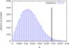 |
Fig. 11 Histogram of dipole amplitudes from 100 000 simulations for the dimensional estimator, assuming the CMB expectation, a slope of x = 0.8, 92,482 sources per simulation and the CG masking form for the WENSS catalogue. The black vertical line is the WENSS result of this work. |
9. Conclusion
We conclude that the task to measure the cosmic radio dipole remains relevant and we expect that interesting information on cosmology can be extracted from this measurement. All measurements so far point towards a higher radio dipole amplitude than expected, when we assume that the cosmic radio dipole is just due to our peculiar motion with respect to the rest frame defined by the CMB. This is quite puzzling, as the orientation of the radio dipole agrees with the orientation of the CMB dipole within measurement errors. This is the case for the NVSS and the WENSS analysis, two radio point source catalogues that cover ~3π and ~π of the sky, respectively. They contain information at different frequencies (1.4 GHz and 325 MHz) and have been put together by different instruments and thus provide a strong constraint on systematic issues.
Our detailed analysis of various linear dipole estimators (Crawford 2009; Singal 2011; Gibelyou & Huterer 2012) for three dimensional estimates (αd,δd,d) and a new linear estimator for a two dimensional estimate (αd,dcosδd) had to tackle several non-trivial issues. We investigated issues of directional bias, amplitude bias and masking. There is still room to optimize the masking of the galaxy. We did not look into quadratic estimators, as used by Blake & Wall (2002). Our studies did not incorporate the uncertainties in point source positions, as we expect that they are subdominant (their magnitude is well below the effect of aberration, see e.g. Rengelink et al. 1997). The measurement error of the flux is also expected to be subdominant as we included sources with flux above 15 mJy only. In the case of NVSS these are a factor 6 above the 5σ point source detection limit, in case of WENSS it is a factor of 1.4. The number of point sources considered in our analysis is about 190 000 for NVSS and 92 000 for WENSS. Putting all those facts together, we consider the NVSS analysis to be more reliable. Nevertheless, the results of the WENSS analysis are fully consistent with our results from NVSS.
Our result (3DS) for the NVSS catalogue is (RA,Dec,d) = (154° ± 19°, − 2° ± 19°,(1.8 ± 0.6) × 10-2). Thus we conclude that the observed amplitude of the radio dipole exceeds the expected amplitude by about a factor of four. We could imagine that this might be due to the structure that causes our proper motion, which in a simple model of our Hubble patch would certainly be aligned with the direction of proper motion. However, all attempts to identify a “great attractor” by means of other observations (optical, infra-red, X-ray) have failed so far. Of all those probes, the radio surveys are definitely the deepest probe of the Universe, as the mean redshift of NVSS sources is estimated to be 1.2 by de Zotti et al. (2010) and 1.5 by Ho et al. (2008). To explain the observed excess radio dipole by contributions from local structure, we would need a density contrast of order 0.05 at scales extending to about z ≈ 0.3, which does not seem plausible. Without a detailed study of the redshift distribution of the radio sources it is impossible to judge whether this finding is actually in agreement with the current standard model of cosmology.
An example of such a scenario is provided by Wiltshire et al. (2012). They claim that the spherically averaged Hubble law on <100/ h Mpc scales is significantly closer to uniform in the Local Group frame as compared to the CMB frame and on this basis have suggested a non-kinematic contribution to the CMB dipole. In this case the CMB dipole could differ from the cosmic radio dipole.
Another reason for the large amplitude of the radio dipole could be that the linear estimators considered in this work do not assume the deviation from isotropy to be a pure dipole. Thus higher multipole moments also contribute to the measured amplitude.
It has been found from the analysis of the CMB that quadrupole, octopole and a few more low ℓ-multipoles seem not to be orientated randomly on the sky, but show some unexpected alignments (Schwarz et al. 2004; Bennett et al. 2011; Copi et al. 2010) among themselves and with the CMB dipole direction. Thus it might not be surprising that also the dominant anisotropy direction of the radio sky lines up.
It is evident that it would be crucial to repeat this investigation with new and even deeper radio catalogues, which provide more sources. In the near future there will be three large sky surveys available (Raccanelli et al. 2012). A multi-wavelength study will be possible based on the Multifrequency Snapshot Sky Survery (MSSS) of the International LOFAR Telescope and with the LOFAR Tier-1 survey. The Australian Square Kilometre Array (SKA) Pathfinder (ASKAP) will produce the Evolutionary Map of the Universe (EMU) and the Westerbrok Synthesis Radio Telescope (WSRT) equipped with the Apertif system will compile the Westerbrok Observations of the Deep Apertif Northern sky survey (WODAN) catalogue.
The multi-wavelength surveys will also allow us to directly measure the spectral index α, which has to be known to connect the measured amplitude to the kinetic dipole. A steepening of the spectral index for the lowest flux sources would increase the expected kinetic amplitude. HI surveys will have the advantage that they will also provide redshift information on top of positions and fluxes and we will be able to study the evolution of the radio dipole as a function of redshift out to redshifts of a few. Beyond that SKA will increase the number of sources in such a survey by orders of magnitude. All these surveys will reduce the random dipole contribution, improve on systematics, and allow us to settle the question: Is the radio dipole in agreement with the CMB dipole?
Acknowledgments
We thank David J. Bacon, Dragan Huterer, Matt J. Jarvis, Seshadri Nadathur, Huub Röttgering and Ashok K. Singal for fruitful comments and discussions and Anne-Sophie Balleier for help with Healpy and the generation of maps of the NVSS and WENSS number counts. The CAMB code, and the Healpy and HEALPix (Górski et al. 2005) packages have been used to estimate the concordance value of the CMB primordial dipole and to produce the NVSS and WENSS maps of the sky. We acknowledge financial support from Deutsche Forschungsgemeinschaft (DFG) under grants IRTG 881 ‘Quantum Fields and Strongly Interacting Matter’ and RTG 1620 ‘Models of Gravity’, as well as from the Friedrich Ebert Stiftung.
References
- Baleisis, A., Lahav, O., Loan, A. J., & Wall, J. V. 1998, MNRAS, 297, 545 [NASA ADS] [CrossRef] [Google Scholar]
- Bennett, C. L., Hill, R. S., Hinshaw, G., et al. 2011, ApJS, 192, 17 [NASA ADS] [CrossRef] [Google Scholar]
- Blake, C., & Wall, J. 2002, Nature, 416, 150 [NASA ADS] [CrossRef] [Google Scholar]
- Condon, J. J., Cotton, W. D., Greisen, E. W., et al. 2002, VizieR Online Data Catalog, VIII/065 [Google Scholar]
- Copi, C. J., Huterer, D., Schwarz, D. J., & Starkman, G. D. 2010, Adv. Astron., 2010, id. 847541 [Google Scholar]
- Crawford, F. 2009, ApJ, 692, 887 [NASA ADS] [CrossRef] [Google Scholar]
- de Zotti, G., Massardi, M., Negrello, M., & Wall, J. 2010, A&A Rev., 18, 1 [Google Scholar]
- Ellis, G. F. R., & Baldwin, J. E. 1984, MNRAS, 206, 377 [NASA ADS] [CrossRef] [Google Scholar]
- Fixsen, D., & Mather, J. 2002, ApJ, 581, 817 [NASA ADS] [CrossRef] [Google Scholar]
- Francis, C., & Peacock, J. 2010, MNRAS, 406, 14 [Google Scholar]
- Garn, T., Green, D. A., Riley, J. M., & Alexander, P. 2008, MNRAS, 383, 75 [NASA ADS] [CrossRef] [Google Scholar]
- Gibelyou, C., & Huterer, D. 2012, MNRAS, 427, 1994 [NASA ADS] [CrossRef] [Google Scholar]
- Górski, K. M., Hivon, E., Banday, A. J., et al. 2005, ApJ, 622, 759 [NASA ADS] [CrossRef] [Google Scholar]
- Hinshaw, G., Weiland, J. L., Hill, R. S., et al. 2009, ApJS, 180, 225 [NASA ADS] [CrossRef] [Google Scholar]
- Hirata, C. M. 2009, J. Cosmol. Astropart. Phys., 9, 11 [Google Scholar]
- Ho, S., Hirata, C., Padmanabhan, N., Seljak, U., & Bahcall, N. 2008, Phys. Rev. D, 78, 043519 [NASA ADS] [CrossRef] [Google Scholar]
- Raccanelli, A., Zhao, G.-B., Bacon, D. J., et al. 2012, MNRAS, 424, 801 [NASA ADS] [CrossRef] [Google Scholar]
- Rakic, A., Rasanen, S., & Schwarz, D. J. 2006, MNRAS, 369, L27 [NASA ADS] [CrossRef] [Google Scholar]
- Rengelink, R. B., Tang, Y., de Bruyn, A. G., et al. 1997, A&AS, 124, 259 [NASA ADS] [CrossRef] [EDP Sciences] [Google Scholar]
- Rubart, M. 2012, Master Thesis, Universität Bielefeld [Google Scholar]
- Schwarz, D. J., Starkman, G. D., Huterer, D., & Copi, C. J. 2004, Phys. Rev. Lett., 93, 221301 [NASA ADS] [CrossRef] [PubMed] [Google Scholar]
- Singal, A. K. 2011, ApJ, 742, L23 [NASA ADS] [CrossRef] [Google Scholar]
- Stewart, J. M., & Sciama, D. W. 1967, Nature, 216, 748 [NASA ADS] [CrossRef] [Google Scholar]
- Wiltshire, D. L., Smale, P. R., Mattsson, T., & Watkins, R. 2012 [arXiv:1201.5371] [Google Scholar]
Appendix A: Monte Carlo simulations
We used the pseudorandom number generator Mersenne Twister for all Monte Carlo
simulations. One simulated source consists of two position coordinates and one flux value.
The coordinates will be drawn from an uniform distribution, leading to an isotropic sky
for a catalogue with many sources. To obtain a desired number count power law like (4) with a certain slope x, we
calculate the flux S using a random number A (choosen
between 0 and 1) by 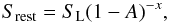 (A.1)where
SL is a flux value 20% below the simulated flux limit. The
simulation also creates sources, which only due to Doppler shifting are counted in the
final catalogue, because this value of SL lies below the
simulated flux limit. Lowering SL further increases
computational time and is not necessary, as long as the simulated velocity
v is below 0.1c.
(A.1)where
SL is a flux value 20% below the simulated flux limit. The
simulation also creates sources, which only due to Doppler shifting are counted in the
final catalogue, because this value of SL lies below the
simulated flux limit. Lowering SL further increases
computational time and is not necessary, as long as the simulated velocity
v is below 0.1c.
The two physical effects (Doppler shift and spherical aberration) will be implemented
separately. In cooperating the Doppler effect is straightforward, since it only affects
the flux values of each source depending on the angle θ between the
source and the velocity direction, i.e.
 (A.2)In the simulation
α is fixed to 0.75 for all sources. The velocity direction and
amplitude can by chosen be the user.
(A.2)In the simulation
α is fixed to 0.75 for all sources. The velocity direction and
amplitude can by chosen be the user.
To model the relativistic effect of stellar aberration one has to change the position of
each radio source. The aberration formula is
 (A.3)where
θ′ is the new angle between the velocity direction and the
radio source. Forth, the position of a radio source is translated into Cartesian
coordinates by assuming that it lies on a unit sphere. Then a straight line from this
point (P) to the velocity direction on the sphere
(V) is constructed depending on a parameter
t
(A.3)where
θ′ is the new angle between the velocity direction and the
radio source. Forth, the position of a radio source is translated into Cartesian
coordinates by assuming that it lies on a unit sphere. Then a straight line from this
point (P) to the velocity direction on the sphere
(V) is constructed depending on a parameter
t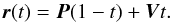 (A.4)On this line we choose a
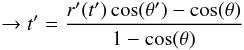
t′ in such a way that
r(t′) points towards the new
position. The value of t′ can be determined by
(A.4)On this line we choose a
t′ in such a way that
r(t′) points towards the new
position. The value of t′ can be determined by
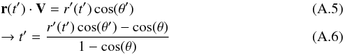
with
 .
This equation is solved by
.
This equation is solved by 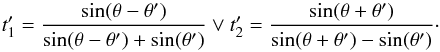 (A.7)We know that for
θ = θ′ the result of
t′ must always be 0. Therefore the correct solution is
(A.7)We know that for
θ = θ′ the result of
t′ must always be 0. Therefore the correct solution is
 . Now one
has to transform r(t′) back into
spherical coordinates in order to find the new position of the radio source. The new
declination ϑ′ is then (the index v stands for the velocity
direction):
. Now one
has to transform r(t′) back into
spherical coordinates in order to find the new position of the radio source. The new
declination ϑ′ is then (the index v stands for the velocity
direction): ![\appendix \setcounter{section}{1} \begin{equation} \vartheta^\prime = \arccos \left(\frac{1}{r^\prime}[(1-t^\prime)\cos(\vartheta)+t^\prime \cos(\vartheta_{\rm{v}})]\right) \vspace*{2mm} \end{equation}](/articles/aa/full_html/2013/07/aa21215-13/aa21215-13-eq534.png) (A.8)and
the new right ascension ϕ′:
(A.8)and
the new right ascension ϕ′:
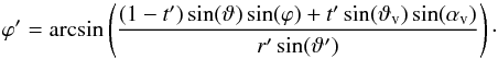 (A.9)This way one obtains a
simulated sky, including the effect of the observers movement. Now one can feed the
different estimators with those sky simulations and obtain the resulting dipole vectors.
(A.9)This way one obtains a
simulated sky, including the effect of the observers movement. Now one can feed the
different estimators with those sky simulations and obtain the resulting dipole vectors.
All Tables
Dipole direction and amplitude from the number count estimator (15) from Singal (2011).
Dipole direction and amplitude from the flux weighted number count estimator (16) from Singal (2011).
Dipole estimate from WENSS based on 2D estimator using peak flux values for all sources with δ > 30°, except those in the Galactic and counter Galactic planes (CG mask).
All Figures
|
Fig. 1 Number counts of the NVSS and WENSS surveys. A function f(S) ∝ S− x is fitted to both data sets in the range of 25 mJy < S < 200 mJy. Resulting values of x are 1.10 ± 0.02 for the NVSS survey and 0.80 ± 0.02 for the WENSS survey. |
| In the text | |
|
Fig. 2 Ampliude bias of the full sky estimator d3D. Data
represent mean and empirical variance of 1000 simulations for each
N. A function |
| In the text | |
|
Fig. 3 Ampliude bias for the estimator d2D on a hemisphere.
Data represent mean and empirical variance of 1000 simulations for each N. A
function |
| In the text | |
|
Fig. 4 Amplitude bias of the 3-dimensional estimator for the masked NVSS geometry of Singal (2011). Data represent mean and empirical
variance of 1000 simulations for each N. A function
|
| In the text | |
|
Fig. 5 Amplitude bias of the 2-dimensional estimator for the masked NVSS geometry of Singal (2011). Data represent mean and empirical
variance of 1000 simulations for each N. A function
|
| In the text | |
|
Fig. 6 Differential number counts of the NVSS catalogue,
Smin = 10 mJy, best fit values for
|
| In the text | |
|
Fig. 7 Map of the number counts in HEALPix pixels from NVSS. The pixel size corresponds to Nside = 32. Shown are equatorial coordinates at epoch J2000. The NVSS contains data at δ > −40° and the Galactic plane and a “counter galaxy” are masked (CG mask) in order to avoid Galactic contamination and to restore point symmetry with respect to the zenith. |
| In the text | |
|
Fig. 8 Map of the number counts in HEALPix pixels from WENSS. The pixel size corresponds to Nside = 32. Shown are equatorial coordinates at epoch B1950. The WENSS contains data at δ > 30° and the Galactic plane and a “counter galaxy” are masked (CG mask) in order to avoid Galactic contamination and to restore point symmetry with respect to the zenith. |
| In the text | |
|
Fig. 9 Differential number counts of the WENSS catalogue,
Smin = 5 mJy, best fit values for
|
| In the text | |
|
Fig. 10 Histogram of dipole amplitudes for 100,000 simulations of the three dimensional (left) and two dimensional (right) estimator, assuming the CMB expectation and a slope of x = 1.1, with 185 649 (left) and 195 245 (right) sources per simulation and appropriate masks. The black vertical lines are the NVSS results of this work. |
| In the text | |
|
Fig. 11 Histogram of dipole amplitudes from 100 000 simulations for the dimensional estimator, assuming the CMB expectation, a slope of x = 0.8, 92,482 sources per simulation and the CG masking form for the WENSS catalogue. The black vertical line is the WENSS result of this work. |
| In the text | |
Current usage metrics show cumulative count of Article Views (full-text article views including HTML views, PDF and ePub downloads, according to the available data) and Abstracts Views on Vision4Press platform.
Data correspond to usage on the plateform after 2015. The current usage metrics is available 48-96 hours after online publication and is updated daily on week days.
Initial download of the metrics may take a while.