© ESO, 2012

1. Introduction

The study of accretion properties of members of star-forming regions (SFRs) is important for our understanding of stellar and planetary formation. While infrared observations provide information on the structure of the circumstellar disk, the accretion properties can be retrieved from photometry and spectroscopy using primary diagnostics, such as UV excess emission (e.g., Gullbring et al. 1998; Rigliaco et al. 2011a), the Paschen/Balmer continuum and Balmer jump (e.g., Gullbring et al. 1998; Herczeg & Hillenbrand 2008; Rigliaco et al. 2011b), or secondary tracers, like hydrogen recombination lines (Hα, Hβ, Hγ, H9, Paβ, Brγ), and the He i, Ca ii, Na i lines (e.g., Muzerolle et al. 1998a,b; Natta et al. 2006; Fang et al. 2009; Rigliaco et al. 2011b; Antoniucci et al. 2011). The rate at which the central star accretes from disk material has been found to approximately scale with the square of the stellar mass and to decrease with age (see, e.g., Herczeg & Hillenbrand 2008, and references therein). In addition, the accretion properties are also important to understand the planet-metallicity relation. In fact, the efficiency of dispersal of circumstellar disks is predicted to depend on stellar metallicity in the sense that the formation of planetesimals around stars is faster at higher metallicity (Ercolano & Clarke 2010). Simultaneous measurements of accretion rates and elemental abundances in SFRs and young clusters are therefore crucial to shed light on the role of metallicity in disk dispersal and planetary formation.

The Chamaeleon II (hereafter Cha II) dark cloud, at a distance of 178 ± 18 pc (Whittet et al. 1997), is one of the three main clouds of the Chamaeleon complex (α ~ 12^h, δ ~−78°). It extends over ~2deg² in the sky (see Luhman 2008 for a recent review). The population of Cha II consists of some 20 classical T Tauri stars (CTTSs), ~ten weak-lined T Tauri stars (WTTSs), an intermediate-mass Herbig Ae star (IRAS 12496−7650; see, e.g., Garcia Lopez et al. 2011), a few Herbig-Haro objects (Alcalá et al. 2008, and references therein), ~three sub-stellar objects, and references therein) and five very low-mass stars (Spezzi et al. 2008, and references therein). Cha II is one of the five SFRs included in the Spitzer Space Telescope legacy program “From Molecular Cores to Planet-forming Disks” (c2d; Evans et al. 2003; Young et al. 2005; Porras et al. 2007). Through extensive work based on c2d IRAC and MIPS Spitzer fluxes and complementary data, a reliable census of the population in Cha II (down to 0.03 M_⊙) was achieved by Alcalá et al. (2008). They concluded that the cloud is dominated by objects with active accretion, with the Class II sources representing ~60%. The same sample was investigated spectroscopically in the optical using GIRAFFE/UVES at the VLT by Spezzi et al. (2008), who derived stellar parameters and estimated a mean age of 4 ± 2 Myr for Cha II. However, studies of radial velocities, elemental abundances, and accretion properties of the cloud members were not addressed in these works. Recently, Alcalá et al. (2011a) analyzed the star IRAS 12556−7731, concluding that it is indeed a background lithium-rich M-giant star unrelated to Cha II.

As a continuation of the studies by Alcalá et al. (2008) and Spezzi et al. (2008), we derive here radial velocities, elemental abundances, and accretion properties for 40 pre-main sequence (PMS) stars in Cha II. The outline of the paper is as follows. In Sect. 2, we describe the spectroscopic observations and data reduction. In Sect. 3, we report determinations of radial velocities, elemental abundances, and accretion properties. The main results are discussed in Sect. 4, while our conclusions are presented in Sect. 5.

2. Spectroscopic observations and data reduction

The observations were conducted in February−March 2006 and February 2007 using FLAMES (GIRAFFE+UVES) at the VLT. A complete journal of the observations and instrumental setup is given in Spezzi et al. (2008). The relevant information for this paper is summarized in Table 1.

We observed 32 objects with GIRAFFE, 11 with UVES, and two with both spectrographs (see Table 1). Despite the ~25′ FLAMES field of view (FoV), it was not possible to assign a large number of fibers in each configuration to the PMS objects/candidates because of the large spatial scatter of the targets. The remaining fibers were allocated to young candidates and field stars¹ (numbers in parentheses in Cols. 4 and 5 of Table 1; see Spezzi et al. 2008 for more details). Thirty-two objects were observed several (2–4) times within two days (see Table 5).

While Spezzi et al. (2008) used a single spectrum per object to derive the spectral type and to confirm the presence of Li i 6708 Å absorption, we use here the complete set of spectra to investigate accretion and short timescale variability. To this aim, we reprocessed the FLAMES/GIRAFFE and FLAMES/UVES observations. The GIRAFFE data were reduced using the GIRAFFE Base-Line Data Reduction Software 1.13.1 (girBLDRS; Blecha et al. 2000): bias and flat subtraction, correction for the fiber transmission coefficient, wavelength calibration, and science frame extraction were performed. Then, a sky correction was applied to each stellar spectrum using the task sarith in the IRAF²echelle package and by subtracting the average of several sky spectra obtained simultaneously. The reduction of the UVES spectra was performed using the pipeline developed by Modigliani et al. (2004), which includes the following steps: subtraction of a master bias, échelle order definition, extraction of thorium-argon spectra, normalization of a master flat-field, frame extraction, wavelength calibration, and correction of the science frame for the normalized master flat-field. Sky subtraction was also performed with the IRAF task sarith using the fibers allocated to the sky.

3. Data analysis and results

3.1. Radial velocity distribution, membership, and binarity

We determined radial velocities (RVs) of each object, choosing Hn 23 and RX J1303.1−7706 as UVES and GIRAFFE templates, respectively. These slowly rotating stars show no strong accretion signatures (see Table 6). We measured the RV of each template (highest S/N) spectrum using the IRAF task rvidlines inside the rv package, which considers a line list. We used 50 and 10 lines for the UVES and GIRAFFE spectra, respectively, obtaining V_rad = 12.5 ± 0.4 km s^-1 for RX J1303.1−7706, and V_rad = 15.2 ± 0.3 km s^-1 for Hn 23. The heliocentric RV of all targets was determined through the task fxcor of the IRAF package rv, which cross-correlates the target and template spectra, excluding regions affected by broad lines or prominent telluric features. The centroids of the cross-correlation function (CCF) peaks were determined by adopting Gaussian fits, and the RV errors were computed using a procedure that considers the fitted peak height and the antisymmetric noise (see Tonry & Davis 1979). When more spectra were acquired, we computed the average RV for each object.

In order to estimate the binary fraction, we considered as singles the stars with only one CCF peak and with night-to-night RV variations within 3σ. In the end, excluding seven objects for which we could not measure the RV, we find six spectroscopic binaries, which means a binary fraction of 18%. In the last column of Table 5, we list the most probable spectroscopic systems. Five stars are newly identified as spectroscopic binaries, while RX J1301.0−7654a was already recognized as a double-lined (SB2) spectroscopic system (Covino et al. 1997).

In Fig. 1, we show the Cha II distribution of the RV measurements in the local standard of rest (LSR) obtained from both the UVES and GIRAFFE spectra, along with the RV distribution of the gas derived by Mizuno et al. (1999) from the C¹⁸O (J = 1−0) transition in 11 dense molecular cores in Cha II. Excluding the spectroscopic binaries, the RV distribution of the Cha II members has a mean of ⟨V_rad⟩ = 11.4 ± 2.0 km s^-1, which translates to a value of ⟨V_LSR⟩ = 4.9 ± 2.0 km s^-1. The Gaussian fit of the distribution yields a mean value peaked at ⟨V_LSR⟩ = 3.9 ± 1.6 km s^-1, i.e. ⟨V_rad⟩ = 10.0 ± 2.1 km s^-1, which is in fairly good agreement with the average velocity of the gas (⟨ V_LSR⟩ = 3.0 ± 0.7 km s^-1, i.e. ⟨V_rad⟩ = 9.6 ± 0.7 km s^-1; Mizuno et al. 1999).

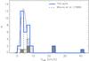Fig. 1 Average RV distribution in the LSR (solid thick line) of the Cha II PMS stars. The distribution of the gas derived by Mizuno et al. (1999) is overlaid (dashed line). The Gaussian fit to the PMS RV distribution is shown (thin line). The shaded histogram represents spectroscopic binary stars, while the hatched one marks the UVES observations. In the case of Hn 24 and Sz 54, where both UVES and GIRAFFE RVs were measured, we considered the UVES observations.

3.2. Lithium equivalent width and radial velocity

Lithium equivalent widths (EW_Li) were measured by direct integration or by Gaussian fit using the IRAF task splot. Errors in EW_Li were estimated in the following way: i) when only one spectrum was available, the standard deviation of three EW_Li measurements was adopted; ii) when more than one spectrum was gathered, the standard deviation of the measurements on the different spectra was adopted. Typical errors in EW_Li are of 0.001–0.087 Å (higher values for GIRAFFE data); for the stars C62 and C66, σ_EWLi ~ 0.15 Å. Our EW_Li measurements are consistent with the values of Spezzi et al. (2008) within 0.02 Å.

Figure 2 shows the EW_Li versus RV for the 37 Cha II members listed in Table 5 (circles) and for the field stars (asterisks). The difference in RV distribution between the no-lithium or weak-lithium stars, and the strong-lithium stars is noticeable. The strong Li stars are confined to a narrow range of velocities (i.e., inside ± 3σ from the peak of the RV distribution). The strong-lithium sample contains single stars and also the two most probable SB1 systems (C66 and IRAS F13052−7653N) and the two SB2 systems (RX J1301.0−7654a and Sz 54), while the rest can be considered as field stars. For the SB2 stars, the average of the RVs of their components falls inside the ⟨V_rad⟩ ± 3σ distribution. The relatively narrow RV distribution of the strong-lithium sample confirms that these stars are all members of the same association.

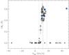Fig. 2 EWLi versus RV for stars in the Cha II FoV (see Table 1). Open circles refer to most probable single stars, filled circles are multiple components, and asterisks refer to field stars. We excluded stars whose binarity was detected from RV variation at different phases (namely, Sz51 and Hn 24; see Table 5). In the case of Sz54, observed with both FLAMES configurations, we considered only the UVES RV values. Vertical lines represent the ⟨Vrad⟩ ± 3σ values, where σ = 2.0 km s-1 (see Sect. 3.1).

3.3. Elemental abundances

3.3.1. Abundance measurements

The FLAMES/UVES wide spectral coverage allows us to select several tens of Fe i+Fe ii lines and spectral features of other elements to measure abundances from line EWs. To this aim, as done in Biazzo et al. (2011b), we discarded stars with T_eff ≲ 4000 K (because of significant formation of molecules in the atmosphere), fast rotators (to avoid rotational blending), and strong accretors (for which accurate abundance analysis is hampered). In the end, only one star (Hn 23) fulfills the required criteria. Effective temperature and surface gravity (log g) from the literature (Table 7) were used as initial values, and initial microturbulence (ξ) was set to 1.5 km s^-1. Final values of the atmospheric parameters are listed in Table 2, together with abundance determinations, abundance internal errors, and number of lines considered (in parenthesis). The first source of internal error in abundance is due to uncertainties in line EWs, while another contribution comes from the uncertainties in stellar parameters. Systematic (external) errors, introduced by the code and/or model atmosphere, are negligible in comparison with the internal ones (see Biazzo et al. 2011a for details on the treatment of errors).

The [Fe/H] value of Hn 23 is slightly below the solar value and in agreement with the mean abundance of ⟨[Fe/H]⟩ = −0.11 ± 0.11 found by Santos et al. (2008) for the Chamaeleon complex (see Fig. 3). This supports the suggestion that SFRs in the solar neighborhood are slightly more metal-poor than nearby young open clusters (Biazzo et al. 2011a). This issue certainly deserves further study, using more stars in the region and homogeneous samples of PMS stars in as many SFRs as possible. Moreover, all other [X/Fe] abundances are close to the solar ones, with silicon and nickel close to the cluster mean value of ⟨[Si/Fe]⟩ = 0.03 ± 0.01 and ⟨[Ni/Fe]⟩ = −0.05 ± 0.02 found by Santos et al. (2008). Titanium seems to be affected by NLTE effects (see Table 2), as previously found by other authors for stars with temperatures cooler than ~5000 K (see, e.g., D’Orazi & Randich 2009; Biazzo et al. 2011a, and references therein). However, detailed treatment of NLTE effects is beyond the scope of this paper.

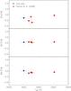Fig. 3 Iron, silicon, and nickel abundances versus spectroscopic temperature for Hn 23 and the stars analyzed by Santos et al. (2008).

3.3.2. Lithium abundance

Mean lithium abundances were estimated from the average EW_Li listed in Table 5 and T_eff values from Spezzi et al. (2008), by using the LTE curves-of-growth reported by Pavlenko & Magazzù (1996) for T_eff > 3500 K, and by Palla et al. (2007) for T_eff < 3500 K. The log g values were derived using the effective temperature, luminosity, and mean mass reported for each star in Spezzi et al. (2008). The main source of error in log n(Li) comes from the uncertainty in T_eff, which is ΔT_eff ~ 100 K (Spezzi et al. 2008). Taking this value and a mean error of 0.020 Å in EW_Li into account, we estimate a mean log n(Li) error ranging from ~0.07−0.10 dex for cooler stars (T_eff ~ 3200 K) down to ~0.05−0.09 dex for warmer stars (T_eff ~ 4200 K), depending on the EW_Li value. Moreover, the log g value affects the lithium abundance, in the sense that the lower the surface gravity the higher the lithium abundance, and vice versa. In particular, the difference in log n(Li) may rise to ~± 0.05 dex when considering stars with mean values of EW_Li = 0.500 Å and T_eff = 4000 K and assuming Δlog g =  ∓ 0.5 dex.

In Fig. 4 we show the mean lithium abundance as a function of the effective temperature (see Table 5 for the log n(Li) values). The average of log n(Li) is about 2.5 dex with a dispersion of 0.6 dex. The lowest lithium abundance values are presumably due to spectral veiling, which affects the line EW.

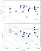Fig. 4 Upper panel: EWLi versus effective temperature. The upper envelope for the Pleiades, as adapted by Soderblom et al. (1993), is overplotted as a dotted line. Lower panel: lithium abundance versus effective temperature. The “lithium isochrones” by D’Antona & Mazzitelli (1997) in the 2–20 Myr range are overlaid with dashed lines. In both panels, empty symbols represent spectroscopic binaries, while mean error bars are overplotted on the lower right corner.

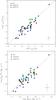Fig. 5 Average ${\mathit{L}}_{\mathrm{acc}}^{\mathrm{H}\mathit{\alpha }}$ (top panel) and $\mathit{Ṁ}\begin{array}{}\mathrm{H}\mathit{\alpha }\\ \mathrm{acc}\end{array}$ (bottom panel) derived from the Hα line as a function of $\mathrm{⟨}{\mathit{L}}_{\mathrm{acc}}^{\mathit{\lambda }}\mathrm{⟩}$ and $\mathrm{⟨}\mathit{Ṁ}\begin{array}{}\mathit{\lambda }\\ \mathrm{acc}\end{array}\mathrm{⟩}$ obtained from the Hβ, He i λ5876 Å, and He i λ6678 Å lines. Mean error bars are overplotted on the lower right corner of each panel.

3.4. Accretion diagnostics and mass accretion rates

The spectral coverage of our data allows us to select several lines (namely, Hαλ6563 Å, Hβλ4861 Å, He i λ5876 Å, He i λ6678 Å, and He i λ7065 Å) that can be used to determine the accretion luminosity (${\mathit{L}}_{\mathrm{acc}}^{\mathit{\lambda }}$). These emission lines are powered by processes related to accretion from the circumstellar disk (Herczeg & Hillenbrand 2008). The use of these lines as secondary accretion diagnostics relies on empirical linear relationships between the observed line luminosity (L^λ) and the accretion luminosity (e.g., Herczeg & Hillenbrand 2008). These relationships have been established through primary diagnostics, such as UV excess emission (Gullbring et al. 1998). We used the ${\mathit{L}}^{\mathit{\lambda }}\mathrm{-}{\mathit{L}}_{\mathrm{acc}}^{\mathit{\lambda }}$ empirical relations of Herczeg & Hillenbrand (2008) to derive ${\mathit{L}}_{\mathrm{acc}}^{\mathit{\lambda }}$. The line luminosity was calculated as ${\mathit{L}}^{\mathit{\lambda }}\mathrm{=}\mathrm{4}\mathit{\pi }{\mathit{R}}_{\mathit{\star }}^{\mathrm{2}}{\mathit{F}}^{\mathit{\lambda }}$, where the stellar radius, R _⋆ , was taken from Spezzi et al. (2008) and the observed flux at the stellar radius, F^λ, was derived by multiplying the EW of each line (EW_λ) by the continuum flux at wavelengths adjacent to the line (${\mathit{F}}_{\mathrm{continuum}}^{\mathit{\lambda }\mathrm{\pm }\mathrm{\Delta }\mathit{\lambda }}$). The latter was gathered from the NextGen Model Atmospheres (Hauschildt et al. 1999), assuming the corresponding stellar temperature and gravity (see Table 7). The mass accretion rate, $\mathit{Ṁ}\begin{array}{}\mathit{\lambda }\\ \mathrm{acc}\end{array}$, was then derived from ${\mathit{L}}_{\mathrm{acc}}^{\mathit{\lambda }}$ using the following relationship (Hartmann 1998): $\mathit{Ṁ}\begin{array}{}\mathit{\lambda }\\ \mathrm{acc}\end{array}\mathrm{=}{\left(\mathrm{1}\mathrm{-}\frac{{\mathit{R}}_{\mathit{\star }}}{{\mathit{R}}_{\mathrm{in}}}\right)}^{-1}\frac{{\mathit{L}}_{\mathrm{acc}}^{\mathit{\lambda }}{\mathit{R}}_{\mathit{\star }}}{\mathit{G}{\mathit{M}}_{\mathit{\star }}}\mathit{,}$(1)where the stellar radius R _⋆  and mass M _⋆  for each star were taken from Spezzi et al. (2008), and the inner-disk radius R_in, when available, from Alcalá et al. (2008). When no R_in was available, we assumed R_in = 5 R _⋆  (see Hartmann 1998), which is a good approximation for most accretors, as pointed out by Alcalá et al. (2011b). Contributions to the error budget on Ṁ_acc include uncertainties on stellar mass, stellar radius, inner-disk radius, and ${\mathit{L}}_{\mathrm{acc}}^{\mathit{\lambda }}$. Assuming mean errors of ~0.15 M_⊙ in M _⋆  (Spezzi et al. 2008), ~0.10 R_⊙ in R _⋆  (Spezzi et al. 2008), and ~0.2 AU in R_in (Alcalá et al. 2008), 5−10% as relative error in EW_λ, 10% in ${\mathit{F}}_{\mathrm{continuum}}^{\mathit{\lambda }\mathrm{\pm }\mathrm{\Delta }\mathit{\lambda }}$, and the uncertainties in the relationships by Herczeg & Hillenbrand (2008), we estimate a typical error in log Ṁ_acc of ~0.5 dex.

Apart from variability phenomena, which will be discussed in Sect. 4.2, the mass accretion rates derived from the various diagnostics should be consistent with each other. In the following, we describe the results drawn from the hydrogen and helium emission lines.

Figure 5 (upper panel) shows the mean accretion luminosity³, derived from the Hα emission line, versus the mean accretion luminosities obtained from other hydrogen and helium emission lines. A fairly good agreement between these diagnostics is present. Comparing the mean mass accretion rate from the Hα line with the mean Ṁ_acc as obtained through the other diagnostics, the agreement is well reproduced (see lower panel in Fig. 5 and Col. 16 in Table 6). This justifies the use of all the diagnostics to compute an average ⟨L_acc⟩⁴ (and, hence, also an average ⟨Ṁ_acc⟩) for each star. A weighted average of ⟨L_acc⟩ derived from the Hα, Hβ, He i λ5876 Å, and He i λ6678 Å emission lines allows us to analyze the relationship between ⟨L_acc⟩ and the luminosity in the He i λ7065 Å line, which is shown in Fig. 6. A linear fit to the relationship gives $\mathrm{⟨}\log {{\mathit{L}}_{\mathrm{acc}}^{\mathrm{He}\mathit{\lambda }\mathrm{7065}}}^{\mathrm{⟩}}\mathrm{=}\mathrm{(}\mathrm{4.01}\mathrm{\pm }\mathrm{0.35}\mathrm{)}\mathrm{+}\mathrm{(}\mathrm{1.14}\mathrm{\pm }\mathrm{0.06}\mathrm{)}\mathrm{⟨}\log {\mathit{L}}^{\mathrm{He}\mathit{\lambda }\mathrm{7065}}\mathrm{⟩}\mathit{.}$(2)The good correlation justifies the use of the He i λ7065 Å line as the reliable diagnostic of L_acc.

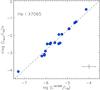Fig. 6 Average accretion luminosity versus line luminosity for the He i λ7065 Å line. The linear fit given in the text (Eq. (2)) is represented by the dashed line. Mean error bars are overplotted on the lower right corner.

As already pointed out, the different line diagnostics yield consistent mass accretion rates (see Fig. 5 and Table 6). Considering, for instance, the Hα line, which is observed in all targets, the mean difference in $\log \mathit{Ṁ}\begin{array}{}\mathrm{H}\mathit{\alpha }\\ \mathrm{acc}\end{array}$ as compared to $\log \mathit{Ṁ}\begin{array}{}\mathrm{H}\mathit{\beta }\\ \mathrm{acc}\end{array}$ is of 0.3 ± 0.3 M_⊙ yr^-1 (with a maximum of 0.8 dex observed for Sz 54), while it is −0.2 ± 0.4 dex with respect to $\log \mathit{Ṁ}\begin{array}{}\mathrm{He}\mathit{\lambda }\mathrm{5876}\\ \mathrm{acc}\end{array}$ (with a maximum of −0.2 dex observed for Sz 56), and 0.1 ± 0.5 dex with respect to $\log \mathit{Ṁ}\begin{array}{}\mathrm{He}\mathit{\lambda }\mathrm{6678}\\ \mathrm{acc}\end{array}$ (with a maximum of 1.1 dex for Sz 50). The mass accretion rate for the sample is in the range 10^-11 ÷ 2 × 10^-8M_⊙ yr^-1, which is typical of Class II low-mass YSOs (see Fig. 2 in Sicilia-Aguilar et al. 2010). Excluding multiple systems, stars with EW_Hα ≤ 10 Å, and the early-type star DK Cha, we find an average mass accretion rate for Cha II of ⟨Ṁ_acc⟩ ~ 7 × 10^-10M_⊙ yr^-1.

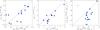Fig. 7 Comparison between our EWHα (left panel), LHα (middle panel), and Ṁacc (right panel) values and those obtained by Antoniucci et al. (2011). In the right panel, mean error bars are overplotted on the upper left corner.

3.4.1. Comparison with previous studies

Fourteen of our targets were also analyzed by Antoniucci et al. (2011) as part of the POISSON (Protostellar Objects IR-optical Spectral Survey On NTT) project aimed at deriving the mass accretion rates of young stars in star-forming regions through low-resolution optical/near-IR spectroscopy. Antoniucci et al. (2011) used the Brγ line as an accretion tracer. They argue that this is the best diagnostic in their spectra when compared with other tracers (i.e., Paγ, Ca ii, Hα, and [O i]). Comparing their log Ṁ_acc with our mean log Ṁ_acc, their values tend to be systematically higher than ours. In particular, their values strongly diverge from ours at log Ṁ_acc < −8, with a mean difference of 1.0 ± 0.8 dex. An analogous trend was found by the same authors when comparing ${\mathit{L}}_{\mathrm{acc}}^{\mathrm{Pa}\mathit{\beta ,}\mathrm{\left[}\mathrm{O}\hspace{0.17em}{i}\mathrm{\right]}\mathit{,}\mathrm{H}\mathit{\alpha ,}\mathrm{Ca}\hspace{0.17em}{ii}}$ with ${\mathit{L}}_{\mathrm{acc}}^{\mathrm{Br}\mathit{\gamma }}$ (see their Fig. 4), which is more evident in their ${\mathit{L}}_{\mathrm{acc}}^{\mathrm{H}\mathit{\alpha }}\mathrm{-}{\mathit{L}}_{\mathrm{acc}}^{\mathrm{Br}\mathit{\gamma }}$ diagram. They ascribe this behavior to enhanced chromospheric emission or absorption from outflowing material, direct photoionization at higher luminosities, or flux losses due to winds.

When comparing the POISSON’s EW_Hα with the values derived by us (left-hand panel of Fig. 7), the difference is ΔEW_Hα = 10 ± 23 Å. Considering that the observations were performed at different epochs (our run was in 2006, while their run was in 2009) and that their EW_Hα were measured on low-resolution spectra (R ~ 700), the agreement is fairly good. In fact, a good correlation is found between our estimated Hα line luminosities and the POISSON’s values, with an average difference of 0.5 ± 0.5 dex in log L_Hα (see Fig. 7, middle panel). Thus, the differences in mass accretion rate arise when deriving L_acc. A similar behavior as the one shown in Fig. 7 for the mass accretion rate is found when our L_acc values are compared with those of POISSON, in agreement with the results by Antoniucci et al. (2011). This means that the differences between POISSON and our determinations are mainly due to the relationships used to derive L_acc. As shown in Fig. 5, very good correlations of L_acc as derived from the He i and Hα lines are found. Should there be an important contribution to the line diagnostics by winds and/or chromospheric activity, our estimates of L_acc would be in excess with respect to those derived from the Brγ line. Instead, the opposite is observed. We thus exclude the possibility that the differences are due to the influence of winds and chromospheric activity. A possible explanation for the difference between our average L_acc values and the POISSON’s ${\mathit{L}}_{\mathrm{acc}}^{\mathrm{Br}\mathit{\gamma }}$ may then be ascribed to the different relationships used to derive L_acc. In order to investigate this issue, measurements of primary accretion tracers, and Brγ measurements are needed. Such analysis cannot be conducted with the data available here, but will be addressed in our future studies exploiting X-Shooter@VLT data (cf. Alcalá et al. 2011b).

3.4.2. Other lines in the optical

A number of optical lines are seen in emission in the spectra of several stars in our sample. These are the forbidden lines of [O i] λ6300.3 Å, and λ6363.8 Å, [S ii] λ6715.8 Å, and λ6729.8 Å, [N ii] λ6548.4 Å, and λ6583.4 Å, as well as Fe ii multiplets. These lines trace mainly stellar/disk winds, jets, disk surfaces, and outflow activity (Cabrit et al. 1990; Hartigan et al. 1995), and their detailed treatment is beyond the scope of this paper. Here, we only note that the [O i] λ6300.3 Å line is detected in 6/11 objects, the [O i] λ6363.8 Å line in 1/11 objects, the [S ii] 6715.8 Å and 6729.8 Å emission is observed in 7/40 and 9/40 sources, respectively, and the [N ii] 6548.4 Å and 6583.4 Å lines are present in 5/40 and 5/40 stars (see Table 5). In the case of Sz 51, the star showing the strongest Hα in our FLAMES/UVES sample, there is evidence of other emission lines (such as the Mg i triplet at λ5167.3, 5172.7, 5183.6 Å, the multiplets 42 and 49 of Fe ii, etc.) indicating mass loss.

4. Discussion

4.1. Accretion versus stellar age and mass

Figure 8 shows the mean mass accretion rate versus stellar age (see Table 7) for all the targets except the early-type star DK Cha, which has a massive disk and high Ṁ_acc (Sicilia-Aguilar et al. 2010). A slightly decreasing trend with age may be present, though over a narrow age interval (~0.4−13.4 Myr) and with a large scatter in Ṁ_acc. This would be consistent with the evolution of a viscous disk (see, e.g., Hartmann et al. 1998; Sicilia-Aguilar et al. 2010, and references therein), although the mean Ṁ_acc is slightly lower than that expected from the model at the Cha II age. In order to quantify the degree of anti-correlation between log Ṁ_acc and log Age, we calculated the Spearman’s rank correlation coefficient using the IDL procedure R_CORRELATE (Press et al. 1996). We find a correlation coefficient ρ = −0.38, with a probability of obtaining such ρ from randomly distributed data of p = 0.08. This seems to confirm a moderate anti-correlation between Ṁ_acc and age, with an average mass accretion rate of ${\mathrm{7}}_{-5}^{\mathrm{+}\mathrm{26}}\mathrm{\times }{\mathrm{10}}^{-10} {\mathit{M}}_{\mathrm{\odot }}$ yr^-1 at a mean age of ${\mathrm{3}}_{-1}^{\mathrm{+}\mathrm{3}}$ Myr. The linear relation we obtain for the likely single stars with mean EW_Hα higher than 10 Å is $\mathrm{⟨}\log \mathit{Ṁ}\mathrm{acc} {\mathrm{(}{\mathit{M}}_{\mathrm{\odot }}\hspace{0.17em}{\mathrm{yr}}^{-1}\mathrm{)}}^{\mathrm{⟩}}\mathrm{=}\mathrm{-}\mathrm{8.84}\mathrm{\pm }\mathrm{0.22}\mathrm{-}\mathrm{0.82}\mathrm{\pm }\mathrm{0.40}\log \mathit{Age} \mathrm{\left(}\mathrm{Myr}\mathrm{\right)}\hspace{0.17em}\mathit{.}$(3)The slope is higher than, yet consistent within the errors with, that obtained by Hartmann et al. (1998) in Cha I (i.e., log Ṁ_acc (M_⊙   yr^-1) = −8.00 ± 0.10−1.40 ± 0.29log Age (Myr)). We warn, however, about the large uncertainties in absolute ages derived from theoretical models for stars younger than ~10 Myr (see, e.g., Spezzi et al. 2008). We note also that a strong constraint on the apparent trend in log Ṁ_acc versus age is set by only one object in the sample (C41, age ~13 Myr). The trend disappears if this object is not considered.

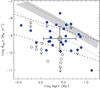Fig. 8 Mean mass accretion rate versus age. Open symbols represent the targets with mean EWHα ≤ 10 Å, while binaries are evidenced as upper limits. The big square represents the mean position of Cha II, taking into account the single stars with mean EWHα > 10 Å (vertical and horizontal error bars correspond to the standard deviations from the mean Ṁacc and age, respectively). The dashed lines mark minimum and maximum limits of Eq. (3), while dotted lines represent the analogous limits of the relationship derived for Cha I by Hartmann et al. (1998). The collection of viscous disk evolutionary models for solar-type stars with initial disk masses of 0.1−0.2 M⊙, constant viscosity α = 10-2, and viscosity exponent γ = 1 reported by Sicilia-Aguilar et al. (2010) is also displayed (filled region).

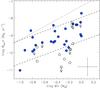Fig. 9 Mean mass accretion rate versus mean stellar mass. Symbols as in Fig. 8. The dashed lines mark minimum and maximum limits of Eq. (4), while the dotted line represents the mean relationship derived for Cha I by Antoniucci et al. (2011). Mean error bars are overplotted on the lower right corner.

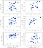Fig. 10 Infrared 2MASS-Spitzer colors versus mean mass accretion rates. Squares and dots correspond to Class III and Class II objects, respectively (see Table 7). Symbol sizes represent stars with EWHα < 10 Å (small squares and dots) and with EWHα > 10 Å (big dots). Mean error bars are overplotted on the lower right corner of each panel.

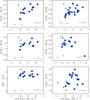Fig. 11 Spitzer-Spitzer colors versus mean mass accretion rates. Symbols as in Fig. 10. Mean error bars are overplotted on the lower right corner of each panel.

Figure 9 shows the mean mass accretion rate versus mean stellar mass (see Table 7). Taking into account single stars with EW_Hα > 10 Å, we find the following linear relationship: $\mathrm{⟨}\log \mathit{Ṁ}\mathrm{acc}\hspace{0.17em}{\mathrm{(}{\mathit{M}}_{\mathrm{\odot }} {\mathrm{yr}}^{-1}\mathrm{)}}^{\mathrm{⟩}}\mathrm{=}\mathrm{-}\mathrm{8.64}\mathrm{\pm }\mathrm{0.21}\mathrm{+}\mathrm{1.30}\mathrm{\pm }\mathrm{0.41}\log {\mathit{M}}_{\mathit{\star }}\hspace{0.17em}\mathrm{\left(}{\mathit{M}}_{\mathrm{\odot }}\mathrm{\right)}\hspace{0.17em}\mathit{,}$(4)where the slope is slightly lower than that found for Cha I (~2; see Antoniucci et al. 2011, and references therein). A correlation of Ṁ_acc with stellar mass is evident. Spearman’s rank correlation coefficient is ρ = 0.51 with a probability p = 0.02. The exponent of the Ṁ_acc − M _⋆  power law is consistent with the range of values ~1.0−2.8 found for low-mass stars in other SFRs (see, e.g., Herczeg & Hillenbrand 2008; Fang et al. 2009; Antoniucci et al. 2011, and references therein).

4.2. Short timescale variability

Young PMS stars are known to be variable, due to the combination of different processes (Herbst et al. 1994) occurring on different timescales: on short timescale (days), variability can be induced by rotation of cool or hot spots (type I variability), and on long timescales (months-years), accretion rate changes (type II variability) or obscuration by circumstellar dust might occur (type III variability, e.g., Schisano et al. 2009). The time span of our observations is ~48 h. Emission line variability on timescales shorter than two days is observed for several objects and for all the analyzed lines (see Fig. B.1). In particular, Figs. A.1–A.3 show the Hα and Hβ profiles of the stars displaying the strongest line variations, while Fig. B.1 shows the mass accretion rates derived from the Hα, Hβ, He i λ5876 Å, and He i λ6678 Å lines versus stellar mass. The vertical bars in these plots represent the range of Ṁ_acc as due to the two-day variability of the corresponding diagnostics.

In general, on the timescale of only two days, the Hα equivalent width of some stars changes up to a factor of 2−3 and, assuming that this is due to accretion, variation in log Ṁ_acc would be 0.2−0.6 dex, i.e., a factor of 1.6−4.0. We conclude that this log Ṁ_acc variability, even if large, cannot explain the log Ṁ_acc spread at a given mass. This means that other stellar properties besides mass must also affect the variations.

4.3. Accretion and metallicity

Investigating the dependency of the mass accretion rate upon iron abundance in SFRs is important for two reasons. First, while the correlation between stellar metallicity and presence of giant planets around solar-type stars is well established (see, e.g., Johnson et al. 2010, and references therein), the metallicity-planet connection in the early stages of planetary formation is still a matter of debate. The evolution of Ṁ_acc is affected by possible planetary formation in the disk, and hence it might provide important clues on the planet-metallicity correlation. Second, the efficiency of the dispersal of circumstellar (or protoplanetary) disks and hence the dispersal timescale are predicted to depend on metallicity in the sense that planetary formation is faster in disks with higher metallicity (Ercolano & Clarke 2010). Yasui et al. (2010) find that the disk fraction in significantly low-metallicity clusters ([O/H]  ~−0.7) declines rapidly in <1 Myr, which is much faster than the value of ~5−7 Myr observed in solar-metallicity clusters. Since the shorter disk lifetime reduces the time available for planetary formation, they suggest that this could be one of the reasons for the strong planet-metallicity correlation.

Recent studies by De Marchi et al. (2011) and Spezzi et al. (2012) in the Large and Small Magellanic Clouds show that metal-poor stars accrete at higher rates compared with solar-metallicity stars in galactic SFRs. Summarizing the mean Ṁ_acc of low-mass (0.1−1.0 M_⊙) Class II stars members of ~3−4 Myr old nearby SFRs for which iron abundance has been recently measured (see Table 3), it is only possible to point out that for [Fe/H]  ~ 0 the mass accretion rate is ~10^-10 M_⊙ yr^-1.

4.4. Fraction of accretors versus age

Excluding the six spectroscopic binaries, 27 of the studied stars result in having mean EW_Hα higher than 10 Å, which would imply a percentage of accretors of about 26/34  =  79% (34 being the total number of single stars in the sample). However, the majority of PMS stars in Cha II have a spectral type later than K7, with most of them later than M3. Therefore, according to the criterion by White & Basri (2003), a more adequate dividing line between most probable accretors and non-accretors in Cha II is EW_Hα = 20 Å. Using this criterion, 19 stars can be classified as true accretors, leading to a percentage of ~55 ± 5%. This fraction of accretors is consistent with the average age of the cloud members. In fact, following the mass accretion rate evolution with time shown in Fig. 3 of Fedele et al. (2010), the fraction of stars with ongoing mass accretion decreases fast with age, going from ~60% at 1.5−2.0 Myr down to ~2% at 10 Myr.

4.5. Color-Ṁ_acc diagrams

Near-infrared colors can be used to probe the inner disk region. Hartigan et al. (1995), studying a sample of 42 T Tauri stars and using the K − L color excesses, pointed out that the disk dispersion is mainly due to the formation of micron-sized dust particles, which combine to create planetesimals and protoplanets at the end of the CTTS phase. Protoplanets may clear the inner disk of gas and dust, causing the disk to lose its near-infrared color excess and at the same time opening a gap in the disk (Lin & Papaloizou 1993), thereby terminating accretion from the disk onto the star.

With the aim of investigating possible relationships between near-infrared colors and accretion properties, we used 2MASS and Spitzer⁵ colors (see Figs. 10 and 11). We considered these colors as disk tracers from the inner to the outer zone because they may estimate the magnitude of the near- and mid- infrared excesses above the photospheric level. In order to quantify the degree of correlation between these diagnostics, we calculated the Spearman’s rank correlation coefficient, as we did in Sect. 4.1, and considered Class II stars with EW_Hα > 10 Å. The correlation coefficients, together with the probabilities, are listed in Table 4 and show that the best agreements are obtained for the Ks−[8.0] and [3.6]−[4.5] colors versus ⟨log Ṁ_acc⟩ parameters. Also, Ks−[4.5], Ks−[5.8], [3.6]−[5.8], and [3.6]−[8.0] colors versus ⟨log Ṁ_acc⟩ show good agreement. This implies that objects with detectable accretion have optically thick inner disks. In particular, we can define the regions where Ṁ_acc > 1.0 × 10^-10 M_⊙ yr^-1 and Ks−[8.0]  >  1.5 or [3.6]−[4.5]  >  0.2, or [3.6]−[5.8]  >  0.5, or [3.6]−[8.0]  >  0.9 as those where accreting objects with infrared excess are found in Cha II. The value Ṁ_acc ~ 10^-10 M_⊙ yr^-1 is a reasonable threshold for the transition from optically thick to optically thin (inner) disk (D’Alessio et al. 2006), as also found by Rigliaco et al. (2011a) in the σ Orionis SFR. The rough trend we tentatively observe among optically thin and optically thick disks, which needs to be confirmed on larger samples, might indicate a link between the mass accretion rate and the grain properties. This link, in turn controls the disk geometry, a connection that is worth exploring further.

5. Conclusions

In this paper, we determined radial velocities, lithium abundances, and accretion properties of 40 members of the Chamaeleon II star-forming region from FLAMES@VLT optical spectroscopy. Elemental abundances of Fe, Al, Si, Ca, Ti, and Ni for a suitable pre-main sequence star of the region were also measured. Our main results can be summarized as follows:

• 1.

  The average radial velocity of the stars is consistent with that ofthe gas (~10−12 km s^-1). The dispersion ofthe radial velocity distributions of the stars and gas (~1−2 km s^-1) are also in agreement.Similar results were found by Dubathet al. (1996) inChamaeleon I (where⟨V_rad⟩_{Cha I} ~ 15.0 ± 0.5 km s^-1).

• 2.

  A binary fraction of 18% is found in Chamaeleon II, which is similar to that in other T associations with comparable star density (see, e.g., the Taurus-Auriga association; Torres et al. 2002).

• 3.

  The metallicity of the suitable member is slightly below the solar value, as also found by Santos et al. (2008) for the Chamaeleon Complex.

• 4.

  We find an average lithium abundance of the star-forming region of 2.5 ± 0.6 dex.

• 5.

  Mass accretion rates derived through several secondary diagnostics (e.g., Hα, Hβ, He i λ5876 Å, and He i λ6678 Å) are consistent with each other, justifying the use of all of them to compute an average mass accretion rate for each star.

• 6.

  We provide a relationship between accretion luminosity, L_acc, and the luminosity of the He i λ7065 Å line.

• 7.

  The relationship between mass accretion rate (Ṁ_acc) and stellar mass (M _⋆ ) in Chamaeleon II is consistent with that found by previous studies in other T associations.

• 8.

  Although slightly lower, the average mass accretion rate in Chamaeleon II fits well the relationship Ṁ_acc versus Age reported by Sicilia-Aguilar et al. (2010).

• 9.

  We cannot exclude that significant variability on timescales longer than the time span of our observations and possibly due to episodes of variable mass accretion may produce the vertical scatter observed in the Ṁ_acc versus M _⋆  plot. However, we suggest that such scatter of about two orders of magnitude in Ṁ_acc at a given mass is also affected by other stellar properties.

• 10.

  The color-Ṁ_acc relationships suggest that the circumstellar disks in Cha II become optically thin at ~10^-10 M_⊙ yr^-1.

• 11.

  The fraction of accretors in Chamaeleon II is ~50%, which, according to the evolution of mass accretion rate in star-forming regions by Fedele et al. (2010), is consistent with the estimated age for the region (~3 Myr).

Online material

Appendix A: Examples of Hα/Hβ line profiles

Here, we display the Hα (Figs. A.1, A.2) and Hβ (Figs. A.3) profiles of the targets showing changes in their line shape and/or intensity. Below, we briefly comment on each object.

Sz 48SW. During the first observing night, the spectrum showed a symmetric, relatively narrow Hα emission profile with a peak close to the line center (type I profile, following the classification of Reipurth et al. 1996). During the second night, the profile appeared slightly asymmetric with lower emission on the blue than on the red side (type IIIB), and then turned back to the type I profile on the third night.

Hn 24. The Hα line profile changes from type IVR (an inverse P-Cygni-like profile) during the first two nights to type IIIR, where less emission in the red than in the blue is seen.

Sz 53. The Hα line shows always a type IIB profile, with a central reversal at the line center and the blue-wing peak intensity lower than the red one. The line strength changes, being maximum during the first observation. The secondary peak always exceeds half the strength of the primary peak. This type of peak is probably due to the interplay of variable accretion and mass loss.

Sz 55. This star shows an Hα line profile changing from IIB to IIIB (where the secondary peak is slightly less intense than half the strength of the primary peak) to IIB.

Sz 57. It always shows a narrow and symmetric Hα emission type I profile with a peak close to the line center.

Sz 58. The Hα profile changes from IIIR (first night) to IIR (second and third night).

Sz 59. IIR/IIR/IIIR profiles are observed for this star during the three observations.

Hn 26. This star shows IIR/IIB/IIB Hα line profiles.

Sz 61. It shows an Hα profile slightly changing from IIB type to IIIB.

Sz 46N. This star shows Hα and Hβ line profiles that are always symmetric (type I).

IRAS 12535-7623. The Hα and Hβ emission line profiles are always consistent with type I.

Sz 50. Its Hα and Hβ emission line profiles are always narrow and almost symmetric (type I).

Sz 51. Hα and Hβ are always of type I.

Sz 56. The Hα profile changes from IIR (during the first and second night) to IIIR (third night), while the Hβ profile is always of type I.

Sz 60W. The Hα line has a complex profile, starting from IIB type during the first night; during the second night, it shows broad wings, red-shifted and blue-shifted absorption, and a narrow emission in the center (like a YY Orion Hα profile, normally associated with high infall and outflow rates, consistent with the high value of Ṁ_acc; Walker 1972); during the third night, it turned back to a IIB type profile. The Hβ line changes from YY Orionis Hβ-like profile to type IIIR to type I.

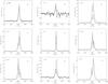Fig. A.1 Examples of Hα emission line profile variations of nine stars. The fluxes are normalized to the continuum. The data refer to the FLAMES/GIRAFFE configuration. The solid/dashed/dash-dotted line represents the first/second/third observation, respectively.

Fig. A.2 Same as in Fig. A.1, but for the UVES data.

Fig. A.3 Same as in Fig. A.1, but for the UVES data and the Hβ profiles.

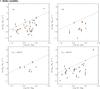Fig. B.1 Mass accretion rates measured from the Hα (left top panel), Hβ (right top panel), He i λ5876 Å (left bottom panel), and He i λ6678 Å (right bottom panel) lines versus mass. Vertical bars connect the minimum and maximum values of Ṁacc obtained per each star at different epochs. Stars are divided into high Hα emitters (EWHα > 10 Å; grey bars) and low Hα emitters (EWHα < 10 Å; orange bars), i.e., stars where the line emission cannot be unambiguously attributed to accretion activity, as it is most likely caused by chromospheric activity. The dashed line shows the relation $\mathit{Ṁ}{}_{\mathrm{acc}}\mathrm{\propto }{\mathit{M}}_{\mathit{\star }}^{\mathrm{1.87}}$ obtained by Herczeg & Hillenbrand (2008) for Taurus members. The highest Ṁacc values in the first and fourth panels refer to the early-type star DK Cha. The lower number of points in the Hβ and He i plots is due to two reasons: absence of the line in the given star or line out of the wavelength range (see Table 5).

Acknowledgments

The authors are very grateful to the referee Ralph Neuhäuser for carefully reading the paper and for his useful remarks. This research made use of the SIMBAD database, operated at the CDS (Strasbourg, France). K.B. acknowledges the funding support from the INAF Postdoctoral fellowship. We thank S. Antoniucci and L. Testi for discussions on accretion luminosity from the Brγ line. We thank G. Capasso and F. Cioffi for their support with the OAC computers. We also thank G. Attusino for his warm assistence during the preparation of the manuscript.

References

All Tables

All Figures

Fig. 1 Average RV distribution in the LSR (solid thick line) of the Cha II PMS stars. The distribution of the gas derived by Mizuno et al. (1999) is overlaid (dashed line). The Gaussian fit to the PMS RV distribution is shown (thin line). The shaded histogram represents spectroscopic binary stars, while the hatched one marks the UVES observations. In the case of Hn 24 and Sz 54, where both UVES and GIRAFFE RVs were measured, we considered the UVES observations.

In the text

Fig. 2 EWLi versus RV for stars in the Cha II FoV (see Table 1). Open circles refer to most probable single stars, filled circles are multiple components, and asterisks refer to field stars. We excluded stars whose binarity was detected from RV variation at different phases (namely, Sz51 and Hn 24; see Table 5). In the case of Sz54, observed with both FLAMES configurations, we considered only the UVES RV values. Vertical lines represent the ⟨Vrad⟩ ± 3σ values, where σ = 2.0 km s-1 (see Sect. 3.1).

In the text

	Fig. 3 Iron, silicon, and nickel abundances versus spectroscopic temperature for Hn 23 and the stars analyzed by Santos et al. (2008).
In the text

Fig. 4 Upper panel: EWLi versus effective temperature. The upper envelope for the Pleiades, as adapted by Soderblom et al. (1993), is overplotted as a dotted line. Lower panel: lithium abundance versus effective temperature. The “lithium isochrones” by D’Antona & Mazzitelli (1997) in the 2–20 Myr range are overlaid with dashed lines. In both panels, empty symbols represent spectroscopic binaries, while mean error bars are overplotted on the lower right corner.

In the text

Fig. 5 Average ${\mathit{L}}_{\mathrm{acc}}^{\mathrm{H}\mathit{\alpha }}$ (top panel) and $\mathit{Ṁ}\begin{array}{}\mathrm{H}\mathit{\alpha }\\ \mathrm{acc}\end{array}$ (bottom panel) derived from the Hα line as a function of $\mathrm{⟨}{\mathit{L}}_{\mathrm{acc}}^{\mathit{\lambda }}\mathrm{⟩}$ and $\mathrm{⟨}\mathit{Ṁ}\begin{array}{}\mathit{\lambda }\\ \mathrm{acc}\end{array}\mathrm{⟩}$ obtained from the Hβ, He i λ5876 Å, and He i λ6678 Å lines. Mean error bars are overplotted on the lower right corner of each panel.

In the text

	Fig. 6 Average accretion luminosity versus line luminosity for the He i λ7065 Å line. The linear fit given in the text (Eq. (2)) is represented by the dashed line. Mean error bars are overplotted on the lower right corner.
In the text

	Fig. 7 Comparison between our EWHα (left panel), LHα (middle panel), and Ṁacc (right panel) values and those obtained by Antoniucci et al. (2011). In the right panel, mean error bars are overplotted on the upper left corner.
In the text

Fig. 8 Mean mass accretion rate versus age. Open symbols represent the targets with mean EWHα ≤ 10 Å, while binaries are evidenced as upper limits. The big square represents the mean position of Cha II, taking into account the single stars with mean EWHα > 10 Å (vertical and horizontal error bars correspond to the standard deviations from the mean Ṁacc and age, respectively). The dashed lines mark minimum and maximum limits of Eq. (3), while dotted lines represent the analogous limits of the relationship derived for Cha I by Hartmann et al. (1998). The collection of viscous disk evolutionary models for solar-type stars with initial disk masses of 0.1−0.2 M⊙, constant viscosity α = 10-2, and viscosity exponent γ = 1 reported by Sicilia-Aguilar et al. (2010) is also displayed (filled region).

In the text

	Fig. 9 Mean mass accretion rate versus mean stellar mass. Symbols as in Fig. 8. The dashed lines mark minimum and maximum limits of Eq. (4), while the dotted line represents the mean relationship derived for Cha I by Antoniucci et al. (2011). Mean error bars are overplotted on the lower right corner.
In the text

	Fig. 10 Infrared 2MASS-Spitzer colors versus mean mass accretion rates. Squares and dots correspond to Class III and Class II objects, respectively (see Table 7). Symbol sizes represent stars with EWHα < 10 Å (small squares and dots) and with EWHα > 10 Å (big dots). Mean error bars are overplotted on the lower right corner of each panel.
In the text

	Fig. 11 Spitzer-Spitzer colors versus mean mass accretion rates. Symbols as in Fig. 10. Mean error bars are overplotted on the lower right corner of each panel.
In the text

	Fig. A.1 Examples of Hα emission line profile variations of nine stars. The fluxes are normalized to the continuum. The data refer to the FLAMES/GIRAFFE configuration. The solid/dashed/dash-dotted line represents the first/second/third observation, respectively.
In the text

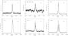	Fig. A.2 Same as in Fig. A.1, but for the UVES data.
In the text

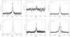	Fig. A.3 Same as in Fig. A.1, but for the UVES data and the Hβ profiles.
In the text

Fig. B.1 Mass accretion rates measured from the Hα (left top panel), Hβ (right top panel), He i λ5876 Å (left bottom panel), and He i λ6678 Å (right bottom panel) lines versus mass. Vertical bars connect the minimum and maximum values of Ṁacc obtained per each star at different epochs. Stars are divided into high Hα emitters (EWHα > 10 Å; grey bars) and low Hα emitters (EWHα < 10 Å; orange bars), i.e., stars where the line emission cannot be unambiguously attributed to accretion activity, as it is most likely caused by chromospheric activity. The dashed line shows the relation $\mathit{Ṁ}{}_{\mathrm{acc}}\mathrm{\propto }{\mathit{M}}_{\mathit{\star }}^{\mathrm{1.87}}$ obtained by Herczeg & Hillenbrand (2008) for Taurus members. The highest Ṁacc values in the first and fourth panels refer to the early-type star DK Cha. The lower number of points in the Hβ and He i plots is due to two reasons: absence of the line in the given star or line out of the wavelength range (see Table 5).

In the text

References

- Alcalá, J. M., Spezzi, L., Frasca, A., et al. 2006, A&A, 453, 1 [Google Scholar]
- Alcalá, J. M., Spezzi, L., Chapman, N., et al. 2008, ApJ, 676, 427 [NASA ADS] [CrossRef] [Google Scholar]
- Alcalá, J. M., Biazzo, K., Covino, E., & Frasca, A. 2011a, A&A, 531, A12 [NASA ADS] [CrossRef] [EDP Sciences] [Google Scholar]
- Alcalá, J. M., Stelzer, B., Covino, E., et al. 2011b, Astron. Nachr., 332, 242 [NASA ADS] [CrossRef] [Google Scholar]
- Allers, K. N., Kessler-Silacci, J. E., Cieza, L. A., & Jaffe, D. T. 2006, ApJ, 644, 364 [NASA ADS] [CrossRef] [Google Scholar]
- Antoniucci, S., García-López, R., Nisini, B., et al. 2011, A&A, 534, A32 [NASA ADS] [CrossRef] [EDP Sciences] [Google Scholar]
- Biazzo, K., Randich, S., & Palla, F. 2011a, A&A, 525, A35 [NASA ADS] [CrossRef] [EDP Sciences] [Google Scholar]
- Biazzo, K., Randich, S., Palla, F., & Briceño, C. 2011b, A&A, 530, A19 [NASA ADS] [CrossRef] [EDP Sciences] [Google Scholar]
- Blecha, A., Cayatte, V., North, P., Royer, F., & Simond, G. 2000, Proc. SPIE, 4008, 467 [NASA ADS] [CrossRef] [Google Scholar]
- Cabrit, S., Edwards, S., Strom, S. E., & Strom, K. M. 1990, ApJ, 354, 687 [NASA ADS] [CrossRef] [Google Scholar]
- Covino, E., Alcalá, J. M., Allain, S., et al. 1997, A&A, 328, 187 [NASA ADS] [Google Scholar]
- D’Alessio, P., Calvet, N., Hartmann, L., Franco-Hernández, R., & Servín, H. 2006, ApJ, 638, 314 [NASA ADS] [CrossRef] [Google Scholar]
- D’Antona, F., & Mazzitelli, I. 1997, Mem. Soc. Astron. It., 68, 807 [Google Scholar]
- D’Orazi, V., & Randich, S. 2009, A&A, 501, 553 [NASA ADS] [CrossRef] [EDP Sciences] [Google Scholar]
- D’Orazi, V., Biazzo, K., & Randich, S. 2011, A&A, 526, A103 [NASA ADS] [CrossRef] [EDP Sciences] [Google Scholar]
- De Marchi, G., Panagia, N., Romaniello, M., et al. 2011, ApJ, 740, 11 [NASA ADS] [CrossRef] [Google Scholar]
- Dubath, P., Reipurth, B., & Mayor, M. 1996, A&A, 308, 107 [NASA ADS] [Google Scholar]
- Ercolano, B., & Clarke, C. J. 2010, MNRAS, 402, 2735 [NASA ADS] [CrossRef] [Google Scholar]
- Evans, N. J., II,Allen, L. E., Blake, G. A., et al. 2003, PASP, 115, 965 [NASA ADS] [CrossRef] [Google Scholar]
- Fang, M., van Boekel, R., Wang, W., et al. 2009, A&A, 504, 461 [NASA ADS] [CrossRef] [EDP Sciences] [Google Scholar]
- Fedele, D., van den Ancker, M. E., Henning, Th., Jayawardhana, R., & Oliveira, J. M. 2010, A&A, 510, A72 [NASA ADS] [CrossRef] [EDP Sciences] [Google Scholar]
- Garcia Lopez, R., Nisini, V., Antoniucci, S., et al. 2011, A&A, 534, A99 [NASA ADS] [CrossRef] [EDP Sciences] [Google Scholar]
- González-Hernández, J. I., Caballero, J. A., Rebolo, R., et al. 2008, A&A, 490, 1135 [NASA ADS] [CrossRef] [EDP Sciences] [Google Scholar]
- Güdel, M., Briggs, K. R., Arzner, K., et al. 2007, A&A, 468, 353 [NASA ADS] [CrossRef] [EDP Sciences] [Google Scholar]
- Gullbring, E., Hartmann, L., Briceño, C., & Calvet, N. 1998, ApJ, 492, 323 [NASA ADS] [CrossRef] [Google Scholar]
- Hartigan, P., Edwards, S., & Ghandour, L. 1995, ApJ, 452, 736 [NASA ADS] [CrossRef] [Google Scholar]
- Hartmann, L. 1998, in Accretion Processes in Star Formation (Cambridge Univ. Press) [Google Scholar]
- Hartmann, L., Calvet, N., Gullbring, E., & D’Alessio, P. 1998, ApJ, 495, 385 [NASA ADS] [CrossRef] [Google Scholar]
- Hauschildt, P. H., Allard, F., & Baron, E. 1999, ApJ, 512, 377 [NASA ADS] [CrossRef] [Google Scholar]
- Herbst, W., Herbst, D. K., Grossman, E. J., & Weinstein, D. 1994, AJ, 108, 1906 [NASA ADS] [CrossRef] [Google Scholar]
- Herczeg, G. J., & Hillenbrand, L. A. 2008, ApJ, 681, 594 [NASA ADS] [CrossRef] [Google Scholar]
- Johnson, J. A., Aller, K. M., Howard, A. W., & Crepp, J. R. 2010, PASP, 122, 905 [NASA ADS] [CrossRef] [Google Scholar]
- Lin, D. N. C., & Papaloizou, J. C. B. 1993, in Protostars and planets III (University of Arizona Press), eds. E. H. Levy, & J. I. Lunine, 749 [Google Scholar]
- Luhman, K. L. 2008, in Handbook of Star Forming Regions Vol. II (ASP Conf.), ed. B. Reipurth, 169 [Google Scholar]
- Mizuno, A., Hayakawa, T., Tachihara, K., et al. 1999, PASJ, 51, 859 [NASA ADS] [CrossRef] [Google Scholar]
- Modigliani, A., Mulas, G., Porceddu, I., et al. 2004, The Messenger, 118, 8 [NASA ADS] [Google Scholar]
- Muzerolle, J., Hartmann, L., & Calvet, N. 1998a, AJ, 116, 455 [NASA ADS] [CrossRef] [Google Scholar]
- Muzerolle, J., Hartmann, L., & Calvet, N. 1998b, AJ, 116, 2965 [NASA ADS] [CrossRef] [Google Scholar]
- Natta, A., Testi, L., & Randich, S. 2006, A&A, 452, 245 [NASA ADS] [CrossRef] [EDP Sciences] [Google Scholar]
- Palla, F., Randich, S., Pavlenko, Y. V., Flaccomio, E., & Pallavicini, R. 2007, ApJ, 659, 41 [Google Scholar]
- Pavlenko, Y. V., & Magazzù, A. 1996, A&A, 311, 961 [NASA ADS] [Google Scholar]
- Porras, A., Jørgensen, J. K., Allen, L. E., et al. 2007, ApJ, 656, 493 [NASA ADS] [CrossRef] [Google Scholar]
- Press, W. H., Flannery, B. P., Teukolsky, S. A., & Vetterling, W. T. 1986, in Numerical Recipes. The Art of Scientific Computing (Cambridge University Press), 489 [Google Scholar]
- Reipurth, B., Pedrosa, A., & Lago, M. T. V. T. 1996, A&AS, 120, 229 [NASA ADS] [CrossRef] [EDP Sciences] [Google Scholar]
- Rigliaco, E., Natta, A., Randich, S., Testi, L., & Biazzo, K. 2011a, A&A, 525, A47 [NASA ADS] [CrossRef] [EDP Sciences] [Google Scholar]
- Rigliaco, E., Natta, A., Randich, S., et al. 2011b, A&A, 526, A6 [Google Scholar]
- Robberto, M., Song, J., Mora Carrillo, G., et al. 2004, ApJ, 606, 952 [NASA ADS] [CrossRef] [Google Scholar]
- Santos, N. C., Melo, C., James, D. J., et al. 2008, A&A, 480, 889 [NASA ADS] [CrossRef] [EDP Sciences] [Google Scholar]
- Sicilia-Aguilar, A., Henning, T., & Hartmann, L. E. 2010, ApJ, 710, 597 [NASA ADS] [CrossRef] [Google Scholar]
- Schisano, E., Covino, E., Alcalá, J. M., et al. 2009, A&A, 501, 1013 [NASA ADS] [CrossRef] [EDP Sciences] [Google Scholar]
- Soderblom, D. R., Jones, B. F., & Balachandran, S., et al. 1993, AJ, 106, 1059 [NASA ADS] [CrossRef] [Google Scholar]
- Spezzi, L., Alcalá, J. M., Covino, E., et al. 2008, ApJ, 680, 1295 [NASA ADS] [CrossRef] [Google Scholar]
- Spezzi, L., De Marchi, G., Panagia, N., Sicilia-Aguilar, A., & Ercolano, B. 2012, MNRAS, 421, 78 [NASA ADS] [Google Scholar]
- Torres, G., Neuhäuser, R., & Guenther, E. W. 2002, AJ, 123, 1701 [NASA ADS] [CrossRef] [Google Scholar]
- Tonry, J., & Davis, M. 1979, ApJ, 84, 1511 [Google Scholar]
- Yasui, C., Kobayashi, N., Tokunaga, A. T., et al. 2010, ApJ, 723, 113 [Google Scholar]
- Young, K. E., Harvey, P. M., Brooke, T. Y., et al. 2005, ApJ, 628, 283 [Google Scholar]
- Walker, M. F. 1972, ApJ, 175, 89 [NASA ADS] [CrossRef] [Google Scholar]
- White, R. J., Basri, G. 2003, ApJ, 582, 1109 [NASA ADS] [CrossRef] [Google Scholar]
- Whittet, D. C. B., Prusti, T., Franco, G. A. P., et al. 1997, A&A, 327, 1194 [NASA ADS] [Google Scholar]
All Tables
Spearman’s correlation coefficients (ρ) and probabilities (p) for different color-Ṁacc relations.